
Table of Contents
Keywords: morphology, plasticity, allocation, mathematical modeling, geometry, hierarchical venation, freeze-thaw mechanism
Abstract
In the interest of optimizing its survival, the maple tree, much like any other living organism, has developed specific biological design solutions. Indeed, the maple tree has evolved over time, developing intricate strategies, described by mathematical features and relationships, that work together to ensure its conservation. Certain species in the Aceraceae arboreal family, including mountain maple, are understory species, meaning they are found in the second layer in forests, where light access can be limited. The mountain maple is characterized by a strong plasticity, allowing it to change leaf size, allocation and growth patterns, ultimately increasing its chances of survival. To understand these changes in morphology, mathematical equations and tools, such as allometric equations, logarithmic transformations, bias-correction factors, linear regression and gradient descent, are used. Furthermore, mathematical modeling using Constrained Delaunay Triangulation (CDT), Voronoi diagrams, 3D interpolation, and the mass-spring can explain how leaf geometry affects the tree's survival. In fact, the distinctive palmate shape and hierarchical venation of the maple leave allow for an even distribution of stress, thereby enhancing leaf stability in unpredictable conditions. Additionally, the maple tree adopts a freeze-thaw mechanism for sap circulation during its dormancy period. This mechanism can be described using a mathematical model that involves differential equations, heat transport equations, multiphase flow models and numerical simulations.
Introduction
The maple tree (Acer) is a symbol of Canadian culture and is a key arboreal feature of forests across North America and Europe, offering aesthetic beauty with its seasonal color changes. The maple has developed personalized strategies and mechanisms that optimize its chances of survival when faced with the harsh conditions of winter. The structural mechanisms and adaptive properties of this tree have been shaped by the problems posed by its environment. Mathematical modeling can describe and explain, in numerical values, the network of geometric patterns, the growth algorithms, and the dynamic processes hidden beneath the maple tree’s seasonal transformations. (see Maple Physics for an extensive introduction)
Understory Maple Species Strategy for Persistence at a Population Level: Case Study of Mountain Maple
Maple trees diverge when it comes to the different layers they occupy in the forests. Shade-tolerant red maple (Acer rubrum L.) trees are often found in the understory of oak forests (Lorimer, 1984). Similarly, Mountain Maple (Acer spicatum) is a common deciduous understory shrub in eastern Canada and northeastern United States (Aubin et al., 2005) .
Forests are generally divided into 4 layers: The emergent layer, the canopy layer, the understory or shrub layer and the floor layer (Fig.1)

Fig. 1. Layers of a temperate forest (Tiffany, 2021).
Although there is uncertainty as to whether the dominance in the understory has a real potential for the tree to become prominent in the canopy (Lorimer, 1984), mountain maple is able to persist across different forest development stages and environments by employing different adaptive solutions. Mountain maple develops as a single stem but can produce basal suckers or shoots when damaged or with age, which leads to forming a dense sub-canopy. As a result, understory light availability is reduced, which impedes the growth and development of seedlings. Mountain maples also benefit from high plasticity, meaning they are able to rapidly respond to environment stresses and change their morphology to better adapt to it. This is hypothesized to favor the persistence of maple trees following major disturbances and in different tree development stages (Aubin et al., 2005).
In order to understand these strategies at a population level, the southern part of the boreal forest of Quebec was chosen as a research forest. It is composed of a mosaic of five post-fire stand development stages: post-fire aspen, mature aspen, mixed wood forest, intact conifer dominated forest and spruce budworm-affected forest. These were chosen to cover a broad range of understory forest conditions (Aubin et al., 2005). Multiple plot specific and mountain maple specific characteristics were determined (Table 1).
Table 1. Characteristics of sampled plots and mountain maple. (a) Percent of basal area of shade-tolerant conifer and aspen in parentheses (b) Light above understory vegetation in parenthesis, PPFD = Photosynthetic photon flux density (c) Biomass determined from equation (6), * subsample used for stem scale analyses (Aubin et al., 2005).

A sample of 100 trees from different understory environments was analyzed in order to determine allometric relationships as well as evaluating the growth and morphological plasticity of mountain maple (Aubin et al., 2005). The dry mass of different parts of the stems was measured, which allowed to determine the leaf area of each stem according to the following relation (Eq. 1):

where is the total leaf area of stem i, is the leaf dry mass of stem i and is the leaf area to dry mass ratio for stem i (Aubin et al., 2005).
Individual stem biomass was estimated from the basal diameter using an allometric relationship (Eq.2) determined from an analyzed sample of 100 trees from different understory environments:

This equation can be logarithmically transformed (Eq.3), yielding:

However, using a non-linear transformation like logarithmic transformation leads to bias in the equation, mainly because a multiplicative error is transformed into an arithmetic error (Packard, 2009). Therefore, a correcting factor must be introduced to account for the bias. This can be calculated from the standard error of estimate SEE, which is calculated as follows (Eq.4):

where are the values of the dependent variable (biomass), and are the corresponding predicted values from the formula. The correction factor can then be calculated (Eq.5):

The corrected formula for the biomass by adding a correction factor of 1.034 is then determined to be the following (Eq.6):

The biomass for the mountain maple (Table 1) were determined using the above equation (Eq.6) (Aubin et al., 2005).
The leaf area and biomass measurements in the sample were used to determine multiple morphological and growth indicators such as Leaf Area Density (LAD), Specific Leaf Area (SLA), Leaf Area Ratio (LAR) and Relative Annual Shoot Biomass Production (Rshoot). The definition and formulae are indicated in Table 2. The variation of these indicators provides information on the plasticity of mountain maple. These indicators have been shown to be a function light contribution and stem height, which relates them to the forest development stage (Aubin et al., 2005). This is done by developing multiple linear regression models that describe the relationship (Eq.7):

where are unknown coefficients, ratio (LAD, SLA…) is the independent variable, Light and stem heigh (Ht) are dependent variables and is the error (Montgomery et al., 2021). Using the different measurements (n=100), this can be put in matrix form (Eq.8):

where y is a vector of the measured ratios, X is a matrix of the measured dependent variables, with the first column being all 1 for the constant coefficient , is the vector of unknown coefficients and is the vector of errors. To get the best regression model, the error must be minimized. This can be done through least-squares regression. We introduce the mean squared loss function (Eq.9):

The loss function is quadratic convex with respect to . The minimum satisfies (Eq.10):

This equation yields (Eq.11):

The parameters can then be determined analytically (Montgomery et al., 2021). However, computing the coefficients using the closed form for big data sizes can be expensive. Therefore, an iterative algorithm known as gradient descent can be used to estimate the least-square coefficients with lighter calculations. The algorithm works by first initializing an arbitrary value for the coefficients, then updating them iteratively as follows (Eq.12):

where is the learning rate. Small numbers for the learning rate are used to achieve stable convergence of the model towards the least-squares coefficients. The components of the gradient of the loss function are as follows (Eq.13):

Note that the sum is the equivalent of a dot product, which is commutative. Since both vectors are column vectors, the matrix form is as follows (Eq.14):

The gradient of the least-square loss function is then (Eq.15):

Operation (12) can be implemented using a programming language such as python (Fig.2), using Equation (15) to calculate the gradient.

Fig. 2. Python implementation of gradient descent algorithm with example values (derivation and code for gradient descent are Rayene’s work)
Using the gradient descent algorithm, the estimated coefficients converge towards constant values that minimize the loss function, yielding the best estimate. Figure 3 shows the evolution of the coefficient value for stem height through iterations in the example given in Figure 2.
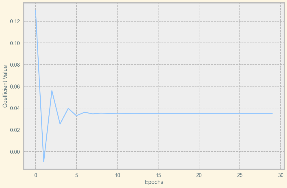
Fig. 3. Stem Height Coefficient evolution through epochs in the example (Rayene’s work).
Using these methods, it is possible to build regression models to find the correlation between the different morphological and growth indicators and the light and stem height (Table 2). In order to evaluate how well-fitted the model is, the Coefficient of determination can be used. It can be calculated as follows (Eq.16 and 17):


is defined as the proportion of variance that is predictable from the independent variables (Chicco et al., 2021), meaning the variance that is not due to the error in the model. R2 values for the regression models for the morphological and growth indicators range from 0.21-0.79 (Table 2). Although these can seem low, it does not necessarily mean the models are inappropriate (Chicco et al., 2021). These models are still pertinent in showing the general trend.
Table 2. Indicators describing stem morphology and growth. A = total leaf area, Mshoot = annual shoot biomass in 1995, CA = crown area, i = of stem i, Mtot = total biomass, Mleaves = leaf biomass, age = age of the plant, Light = light above the understory vegetation, Ht = stem height,* All the regression models are significant at P<0.001, R2 are adjusted (Aubin et al., 2005).

The different points used for the regression model are plotted in a scatter plot as both a function of light and stem height (Fig. 4.).

Fig. 4. Relationships between maple crown morphological and growth ratios (a) LAD, b) LAR, c) SLA, d) Rshoot) and light above the understory vegetation (PPFD%). Dot size is a function of stem size(Aubin et al., 2005).
Stem growth and crown morphology are influenced by both light conditions and stem height. At high light intensity, smaller and thicker leaves and a higher leaf area are believed to maximize light interception and growth, which is shown in the low SLA and high LAD at high PPFD, although growth seems to decrease above 60% PPFD, which matches with previous descriptions of optimal conditions for mountain maple growth(Aubin et al., 2005). LAR is negatively proportional to stem height at all light levels. Thus, an increase in size at low light will induce a carbon stress (metabolic imbalance) in mountain maple, and maintaining a small size increases its chance of survival. Rshoot increases with increasing light, reaching optimal growth at 60%. These light requirements are characteristic of gap-phase strategy. Both light availability and stem height must therefore be considered to explain mountain maple’s strategy to survive in different understory environments (Aubin et al., 2005).
Four distinct phases of mountain maple dynamics are proposed based on the stands studied (Aubin et al., 2005).
The post-disturbance (clearcut or fire) removal of aboveground vegetation leads to a rapid growth of young stems favoured by multi-layer morphology with high LAD. This stage is observed in the young aspen forests
As aspen forests get more mature, mountain maple tends to increase in density, size and overall biomass. During this expansion phase, mountain maple may increase in abundance and colonize the understory.
An increase in the number of shade-tolerant conifer trees in the overstory canopy tends to reduce light in the mixed wood understory regions to below 10%. This is detrimental to mountain maple density, biomass and height. Mountain maple’s morphology adapts and takes on a shade-adapted form with monolayers and a height decline.
The increase of budworm host species in the canopy makes the forest prone to gap formation. Following small-scale disturbances such as these gaps, mountain maple can quickly occupy the openings and rapidly forms a dense sub-canopy with high biomass and more high stems.
Mountain maples are therefore able to quickly alternate between suppression and expansion depending on the conditions, ensuring its persistence (Aubin et al., 2005).
Leaf Modelling
Maple trees (Acer) belong to a major group of flowering plants called dicotyledons (‘dicots’). Their leaves usually exhibit a netlike venation pattern, as opposed to monocotyledons (‘monocots’), whose veins are typically arranged in parallel (Ersek, 2012). For most dicot leaves, structural stability depends on low-order veins; namely primary, secondary, and tertiary veins (Hong, 2005). Secondary veins branch out from primary veins, and tertiary veins branch out from secondary veins, and so forth. This particularly applies to maple leaves, which possess a palmately lobed and thin structure, meaning it has several large lobes which all radiate outwards, increasing mechanical complexity. The maple leaf’s venation skeleton impacts the way the entire leaf moves and reacts to deformation. A large lobed lamina like the maple leaf with thin and minimal material must resist aging, non-uniform bending, and unpredictable deformation under unpredictable weather conditions like wind. Non uniform and random deformation to the leaf can result in it being more susceptible to drag, damaged transport pathways, tearing, and a drop in sunlight capture and a decreased total surface area for photosynthesis, which is essential for the survival of the tree (RHS Gardening, n.d.). Hence, structural support must be distributed efficiently with minimal mesh. This section of the paper will utilize mathematics to model and visualise how the maple leaf’s venation structure helps distribute stress.
The venation skeleton of a maple leaf can be described as a hierarchical tree structure branching radially from a central node at the petiole (Fig. 5). Each lobe contains a primary vein, with secondary and tertiary veins branching out from it, reinforcing the lamina.

Fig. 5. External structure of a dicotyledon leaf (Hong, 2005).
This allows for equal and uniform distribution across the lamina, with the hierarchical branching (Fig. 6) controlling bending at different scales. This is because deformation that affects low order veins affects the entire lamina. This radial spread of low order veins forms a tree topology that results in smooth deformation, allowing maple leaves to bend gracefully due to their unique geometric arrangements.

Fig. 6. Venation skeleton modelling of a maple leaf (Hong, 2005).
To analyze the efficiency of the maple leaf’s venation structure and how its skeleton supports the lamina, the leaf surface can be modeled using Constrained Delaunay Triangulation (CDT), which divides the leaf into connected triangles following the leaf’s skeleton, with mesh between the triangles (Fig. 7). This mathematical model also maximizes the minimum internal angle of each triangle, preventing skinny, unstable triangles which would simulate unrealistic deformation. This is an accurate and realistic way to predict and simulate the deformation of a maple leaf based on its skeletal geometry, and accurately reflects how unstructured mesh conforms to complex environmental loads (Hong, 2005).

Fig. 7. Delaunay Triangulation of a maple leaf with different size constraints (Hong, 2005).
Figure 7 displays two triangulations of the maple leaf generated with different size constraints: 1000 and 400 for (a) and (b) respectively, where ‘p’ stands for pixel and is the area in pixel units. In the 1000 diagram, the mesh displays irregular, elongated triangles, creating an uneven surface curvature. Whereas the 400 diagram possesses smaller and more uniform triangles, resulting in a smoother deformation pattern (Hong, 2005).
The Delaunay triangulation models can also be interpreted as Voronoi regions, which define how force from veins spreads across the lamina. Each triangle’s circumcenter corresponds to a Voronoi vertex, allowing efficient computations from the triangulated mesh. In the below formulation, natural-neighbor interpolation is described by (Eq.18):

Where is the interpolated function value, are the data values at the natural neighbor nodes to the point, and corresponds to how much influence the neighboring vein node has on the value (Sambridge et al., 1995). This equation can be used to predict the interpolated deformation at any point in the lamina, highlighting the mathematical principle of how the maple leaf’s venation structure behaves like an optimized interpolating system. No point on the lamina acts in isolation, as its stress depends on nearby veins, demonstrating how the leaf behaves as a continuous system where forces are smoothly distributed across the leaf, as opposed to concentrated deformation at specific points. This mathematically reflects the structural optimality of the maple venation network, which increases mechanical stability and helps prevent localized tearing or nonuniform folding under the harsh and unpredictable weather conditions maple trees are often exposed to (Oswald et al., 2018).
Figure 8 illustrates the interpolation of leaves in 3D, which shows how the nodes’ positions along the lamina can be interpolated to reconstruct a realistic curved surface. It visualizes how the 2D leaf domain (Ω) is extended into a smooth 3D surface by interpolating (x,y,z) coordinates at each mesh node. The dashed red lines connect to nodes with fixed boundary values along primary veins, while surrounding regions are freely interpolated, creating a continuous curvature along the lamina. Incorporating a 3rd dimension increases numerical accuracy, with boundary conditions applied along the main veins, smoothening the transition between constrained and unconstrained regions. This shows that the maple leaf can be mathematically interpreted as a 3D continuous function, facilitating a more precise simulation of its deformation behavior.

Fig. 8. Interpolation of leaf coordinates in 3D (Hong, 2005).
Table 3 quantifies how reducing the maximum allowable triangle area in a Constrained Delaunay Triangulation results in increased surface stability across the lamina and more uniform deformation. As the maximum square-pixel size was reduced from 1000 to 300, the number of triangles increased, alongside the number of nodes and edges, resulting in a more uniformly connected mesh structure. This reduces geometric irregularities, allowing for a more mathematically accurate exhibition of curvature under load. This data confirms the behavior of the maple leaf’s venation pattern as a mathematically optimized lattice and further reinforces the biological optimization of the maple leaf, whose unique geometric pattern achieves maximum stability with minimal material.
Table 3. Effects of maximum triangle area constraint on triangulation (Hong, 2005)

Furthermore, the maple leaf’s palmately lobed geometry contributes to its structural efficiency. According to the observed deformation due to aging in Figure 9, only distal lobes tend to curl, while the central lamina where the low order veins are concentrated remains planar. This selective deformation can be attributed to the maple leaf’s unique geometry and radial branching pattern. From a mathematical perspective, this partition results in almost triangular structures branching from the central node, minimizing strain, and maximizing the area unaffected by deformation (Sack et al., 2008), leaving more total surface area for sunlight capture for performance of photosynthesis and other metabolic processes.

Fig. 9. Maple leaf aging phenomena (Hong, 2005).
Moreover, the mass-spring model is also often used to simulate the deformation of soft fabrics. There are two essential components to this model: a series of virtual particles and the corresponding light springs of a nonzero length. Hence the triangulated mesh model of a maple leaf can be used as a mass-spring model, where the vertices are treated as particles, and the edges as springs. The joint forces (internal and external forces acting on the spring) will be denoted as Fi,j(t) . This model provides a dynamic mathematical framework to simulate and approximate how the maple leaf’s skeletal structure responds to external forces. The system follows Newton’s laws, and the equations to calculate the acceleration, velocity, and displacement of particles are(Eq.19,20 and 21):


Where corresponds to the mass of the particle, ai,j represents its acceleration, the time step is denoted by Δt (must be small to ensure numerical stability in the calculations), and vi,j and Pi,j correspond to its velocity and displacement, respectively (Tang et al., 2013). A velocity constraint was introduced to prevent over-elasticity, as the deformation of the leaf under forces is not ideally linear, and the deformation of the springs could exceed 100%. Hence, a constraint condition is introduced, ensuring that each spring cannot elongate more than 10% of its natural length (τc = 0.1). In the following equation (Eq.22):

“L” represents the natural length of the leaf vein (spring) without any forces exerted, and τc is the threshold of deformation. When τc is set to equal 0.1, this equation guarantees that the maximum length of the spring does not exceed 10% of its initial natural length (Tang et. al., 2013). This mathematically delineates how maple leaves don’t stretch indefinitely despite bending and twisting, and that the venation structure of the leaf redistributes and localizes strain.
To conclude this section, the mathematical models such as Delaunay triangulation, Voronoi diagrams, and the mass-spring model that were explored reveal how the maple leaf’s venation structure acts as a continuous, optimized and adaptive system, overcoming everyday engineering challenges by maximizing stability with minimal material over a venation skeleton, preserving surface integrity. The maple leaf has evolved to possess a unique set of geometrical and mathematical features under its belt, including its palmately lobed lamina and radial branching, which compartmentalize deformation and increase structural stability. This adaption allows maple trees to cope with everyday problems posed by mother nature, as its leaves have evolved to handle stress with minimal deformation due to their unique geometry, keeping transport pathways open, a maximized surface area for photosynthesis, and functional, healthy, and resilient leaves which can perform the necessary metabolic functions for the tree to survive. The maple leaf is a complex and inspiring system from which engineers can learn a lot from, including applications for biomimetic design of anything ranging from flexible architectural facades to wind resistant solar panels.
Sap Flow Modelling
Sap flow in maple trees varies depending on the season. During the growing season, the sap travels through a process called transpiration: 90% of the water stored in the roots is transpired through the leaf stomata, while the remaining 10% is used for photosynthesis reactions (Ceseri & Stockie, 2013). The carbohydrates formed are dissolved in sap as sucrose, and are transported through sapwood, allowing the nutrients to reach cells across the tree. The carbohydrates are then used for structural and metabolic necessities, while some are stored as starch for later use. Among the different purposes, the stored starch serves as an energy source during the leafless period in spring for leaf and bud growth. Stored starch transforms into soluble sugars and is released into sap circulating in the tree. However, since the tree doesn’t have any leaves to generate transpiration-induced flow, it must rely on different processes to move sap and provide the necessary sugars to cells responsible for leaf and bud growth (Ceseri & Stockie, 2013). Maple trees, specifically Acer Saccharum (sugar maples) and Acer Rubrum L. (red maple), are known for their outstanding ability to generate sap exudation during this period (Ceseri & Stockie, 2013; Zarrinderakht et al., 2024). It took many years for scientists to understand this phenomenon, though it remains misunderstood. The foundational study that first contributed to the understanding of sap exudation was that of Milburn and O’Malley. They proposed a model of sap flow based on a freeze-thaw mechanism. Sap flow during the leafless period relies on variations of temperatures about the freezing point between the warm days and cold nights of spring. The tree cells contain sap (or water) and gas bubbles. Pressure changes caused by the oscillating temperatures lead to the movement of sap, mainly in the longitudinal direction. In more details, as illustrated in Fig. 10, when temperatures decrease below the freezing point, water in fibers gradually freeze, and the gas contained within them contract, causing a negative pressure that causes sap to move upwards. Then, when temperature increase, the water melts (thawing), gas bubbles expand and the resulting positive pressure leads sap to flow back downwards. Essentially, the freeze-thaw cycles (Fig. 11), combined with pressure changes of gas bubbles within the tree cells, caused by temperature changes, was theorized to be the root cause of sap exudation. This theory was confirmed through multiple experiments. However, the Milburn and O’Malley model couldn’t explain why the gas bubbles wouldn’t dissolve, which would in that case inhibit the freeze-thaw action. Not long after, several studies suggested the presence of an osmotic pressure that would prevent this by decreasing the pressure acting on the gas bubbles. The correlation between sugar content in sap and exudation has been confirmed through experiments. However, the importance of the osmosis effect, which has been discussed in Maple Chemistry, is still debated. Additionally, other mechanisms are suspected to influence sap flow during spring. Therefore, even with both theories, sap exudation cannot be fully explained yet. This might be due to absence of a mathematical model of combined mechanisms. Recent papers describe sap exudation mathematically, using derived differential equations to describe the multiphase gas/liquid/solid system and study the effect of the different physical mechanisms. A model incorporating the thawing sap, the osmotic gradient, and the osmotic pressure can bring light to this issue. Additionally, numerical simulations are used to confirm whether the mathematical model accurately depicts the movement of sap. Finally, with the combination of both methods, conclusions can be formulated regarding the role of mechanisms in sap flow (Ceseri & Stockie, 2013).

Fig. 10. 2D simplified illustration of the freeze-thaw mechanism. The cooling sequence starts with the loss of heat, caused by decreased temperatures (1). The gas bubble within the fibre contracts and water enters the fiber and freezes leading to negative pressure that causes root uptake (2), until freezing of sap is complete (3). Then, in the warming phase, as sap melts and the gas expands, positive pressure inside the fiber causes the sap to enter the vessel, thus causing downwards flow of sap (4) (Graf et al., 2015).

Fig. 11. Illustration of the movement of water within a tree stem through each step of the freeze-thaw process described in Fig. 10 with associated temperature variations. The gas bubble reaches its maximum volume when temperatures peak, and the water is fully melted (i). As temperatures decrease, the gas bubble contracts and entering water freezes (ii). Minimum temperatures cause the liquid in fibers to fully freeze (iii). Finally, increasing temperatures melts the water, allowing the gas to expand. (iv) The arrows represent the thawing and freezing fonts. Thin annular regions in ii) and iv) (grey area separating the gas-water interface) represents the thin freezing (ii) and melting (iv) water layer (Zarrinderakht et al., 2024).
Step 1. Description of Sapwood Anatomy
First, to schematize the model, it is essential to consider the structure of the xylem (Fig. 12). The xylem is composed of vessels and fibers. These cells are cylindrical-shaped, long and hollow. Their length, which varies in the dozens of centimeters, stretches along the longitudinal direction of the tree. Fibres are mostly gas-filled, and are the main structural element of wood, while vessels have a bigger radius, and are the conduits where sap moves along depending on the pressure. Pits can be found in connecting vessels to each other. A semi-permeable membrane (with only water permeability) separates vessels from fibers and is responsible of osmosis pressure effects. For simplification purposes, only the thawing step of the process (step 3 and 4 in fig. 10 or iii) and iv) in Fig. 11) will be described by the differential equations (DEs) used (Zarrinderakht et al., 2024).

Fig. 12. (a) Illustration of a section of Xylem, the maple tree’s matrix. The vessels have larger radii compared to fibers, which surround vessels. The pits serve as hydraulic connexions. (b) Defined dimensions length and radius ({Lf, Rf} and {Lv,Rv} of the fiber and the vessel respectively (Zarrinderakht et al., 2024).
Step 2: Define the Unknown Functions
The main variables used for the governing equations are presented in Table 4. The model equations are essentially the same as those presented in Graf et al. (2015), and complete details of the derivation can be found there and in Ceseri and Stockie (2013). The physical state of the various phases (liquid, ice, gas) within a given vessel and fiber pair can be described by the following six time-dependent functions (Zarrinderakht et al., 2024). Fig. 13 illustrates radii and interface geometric parameters used in the model, thus allowing a quantitative description of sap movement in and out of the cells (Equ 23-25).
Table 4. Main functions described by the governing differential equations (Zarrinderakht et al., 2024).
| siw(t) | fiber gas bubble radius, measured from the center of the fiber (fig. 4) |
|---|---|
| sg(t) | radius of the fiber ice-water interface (fig. 4) |
| r(t) | vessel gas bubble radius (fig. 4) |
| U(t) | total volume of meltwater that flows through the porous fiber–vessel wall, measured positive from fiber to vessel (fig. 4) |
| Ur(t) | total volume of water influx from the roots |
| Τ(y,t) | temperature in the vessel sap, which depends on the radial coordinate y with origin at the vessel center so that r(t) ≤ y ≤ Rv |

Fig. 13. Schematic representation of the simplified vessel-fiber unit cross-section showing key geometrical parameters used in the DEs (Ceseri & Stockie, 2013).
Step 3. Define Main Differential Equations
First, the unknown time-only dependent functions are described. Starting with an algebraic equation of conservation of volume, an ODE can be defined, describing the thickness of the layers within the fibre (all radii of each phase) in relation with the water travelling from the fibre to the vessel U(t) (Eq.23):

The variables ϱw and ϱi represent the water and ice density respectively.
Similarly, the volume conservation equation describes the vessel gas bubble radius r(t) (Eq.24):

The function describing the ice-water interface throughout time siw(t) is derived from the Stefan condition, which describes the change of the interface related to the change of phase (Eq.25):

where kw is the thermal conductivity of water, and Ew-Ei is the latent heat. ∂nT=∇yT·n, the normal heat flux.
Darcy’s law describes the flow rate of an incompressible fluid. Using this law, the rate of change of U and Ur, with regards to time, can be described as (Eq.26):

And (Eq.27):

with L and Lr are the hydraulic conductivity and the root hydraulic conductivity respectively, pvw pfw are the liquid pressures of the fibre and the vessel respectively. Cs is the osmotic pressure due to sugar concentration gradients, and Ѱs is the pressure balance (water potential difference between water and soil).
Equations 23-27 describe the dynamics within the fiber and vessel during a thawing cycle only. Three additional equations describe algebraic constraint of the previous equations. These include a sap pressure equation, which includes the balance between gas pressure and surface tension pressure at the gas-bubble interface, the gas density, and the cell water volumes. These ODEs can be adapted to depict every step of the freeze-thaw process (Fig. 14). A homogenized two-scale model provides two heat-diffusion equations governing heat transport. The first equation captures the microscale effects resulting from phase change in the cells, while the second describes the macroscale effects caused by ambient temperature fluctuations. Other equations used allow the regulation of more detailed and more complex effects. It is also worth highlighting that these equations include other factors influencing the sap flow mechanism, which haven’t been properly theorized yet, like the freezing point depression (FPD), that are proven with numerical simulations to have a significant influence (Zarrinderakht et al., 2024).

Fig. 14. Phases of the freeze-thaw mechanism with their associated governing differential equations in the microscale. The equations for pif, ∂tsiw, and ∂tsg, represent the capillary pressure, the changing ice-water interface and the changing radius of the gas bubble respectively. These equations vary according to the freeze-thaw phase. Specifically, the ∂tsiw, and ∂tsg equations are adapted formulas of Equation 23 and Equation 25 (Graf & Ceseri, 2015).
Numerical Simulations
Numerical simulations were used to compare experimental data on sap flow throughout the freeze-thaw period and compare it to the simulated homogenized model. The homogenized model, which consists of derived microscale equations, combined with macroscale equations describing heat transport took into considerations both theories on sap exudation, describes accurately the mechanisms taking place in sapwood. In fact, experiments ran on two red maples (R1 and R2) and a sugar maple (S1), tracked the pressure fluctuations with respect to temperature changes throughout the leafless season, a period of 27 days (Fig. 15). When compared to the homogenized model, very few differences in these parameters were observed. As a result, modeling sap flow of leafless season trees as prov-+en to be effective in predicting the behavior of sap throughout the season. Moreover, the model allows to draw conclusions on which phenomena exert a significant influence on sap flow (Zarrinderakht et al., 2024).

Fig. 15. Comparison of experimental stem pressure and simulations for the red maples (a and b), and the sugar maple tree (c). The solid-blue lines represent the simulations, while the dashed light-blue traces represent experiments. The black smooth line represents the smoothed temperature data. Each freeze thaw event (completed cycle), defined as the moment when temperatures cross 0°C (step iv in Fig. 11, or 1 in fig. 10), is highlighted with the black vertical dashed lines. At the same time, in experiments, spikes in pressure occur, (which aren’t as defined in the mathematical simulation). Weak freeze-thaw events, which were detected in red maples, are highlighted inside a red-edged frame (Zarrinderakht et al., 2024).
Design Solutions
First, comparison between experiments and simulations demonstrated that a physical model (freeze-thawing) can capture the pressure changes observed. Four mechanisms were also identified to be generating stem pressure buildups. The unique cellular structure of maple sapwood provides a mechanism of fiber-vessel pressure exchanges. The layout of fibers surrounded with vessels, with whom they share a semi-permeable separating membrane allows liquids to be drawn into the fiber due to negative pressure caused by freezing water, attracting pure water into the fiber (cryostasis suction). Second, the sugar content of sap affects the freeze-thaw pressure generation through the significant osmotic potential between the fiber and the vessel, preventing the dissolution of gas bubbles and thus maintaining the pressure exchange between the two cells. The FPD (freezing point depression), an additional physical effect, influences the system much more significantly. The average FPD of a maple with 3% sugar content is roughly -0.16°C. In other words, sugar content in sap lowers the freezing temperature of sap which causes efficient water accumulation from the vessels into fibers during the freezing stage, as well as maintaining the sugary sap in vessels liquid. Furthermore, the heat transport only affecting the system on the macroscopic scale allows thawed vessels to be surrounded by partially frozen fibers. Lastly, the presence of liquid water in the soil allows efficient movement of water upwards despite freezing temperatures, thereby accumulating and freezing in fibers during the cooling phase, which increases the pressure acting on the gas bubble for efficient ejection of water in the vessel during thawing, and hence maintaining optimal exudation (Zarrinderakht et al., 2024).
Essentially, mathematical models and numerical simulations enable the evaluation of the contribution of physical mechanisms, and to what extent each one matters. Multiple mechanisms have been discovered and explained in isolation. Consequently, building a quantitative model integrating all theories and comparing it to experiments allows a more comprehensive and realistic study. The four design solutions have all been included in the equations, which resulted in a realistic behavior of the model. However, one design omitted would be sufficient to cause model failure to match the pressure dynamics of the experimental behavior (Zarrinderakht et al., 2024).
Conclusion
A wide range of mathematical equations and models can be applied to the strategic efforts adapted by the maple tree to ensure its survival in the face of stressors. Indeed, understory maple species like the mountain maple can adjust leaf morphology based on external conditions. Mathematical tools such as allometric equations, logarithmic transformations, bias-correction factors, linear regression and gradient descent are used to measure and interpret the relationships between leaf area, stem height, stem biomass and light availability. Thus, the following conclusions were made, linking different leaf morphologies to the forest’s growth phase:
In young aspen forests, the mountain maple leaves expand rapidly following an environmental disturbance.
As aspen forests begin to mature, mountain maple trees increase in density and height.
With an increase in conifers, there is less light that reaches the understory level, and the mountain maple reduces in size, adopting its shade-adapted form.
As the aspen forest adopts a gap formation, the mountain maple the small gap, causing a rapid regrowth characterized by an increase in density, biomass and height.
Therefore, in the interest of population persistence, the mountain maple can quickly alternate between suppression and expansion states. Moreover, maple leaves have hierarchal venation and a palmate shape, ensuring structural optimization by distributing stress and increasing stability. This structural efficiency allows the leaf to maintain surface area for photosynthesis, to resist tearing, to reduce uneven bending and to effectively distribute mechanical stress. Mathematical modelling can explain the efficiency of the leaf's geometry and vein branching. In fact, Constrained Delauney Triangulation (CDT) and Voronoi diagrams show how the division of the leaf’s surface into small triangles allows for smooth deformation and distribution of forces. 3D interpolation reveals how the leaf undergoes deformation and the mass-spring model reveals the leaf’s structural resilience. Finally, after losing its leaves, the maple tree uses a freeze-thaw mechanism for sap exudation. To fully understand this mechanism a mathematical model was created involving melting ice, osmotic gradients, gas bubble mechanics, water movement across membranes and heat diffusion. This model produced numerical simulations describing the sap’s circulation that closely resemble real measurements from maple trees. The maple tree adapted this mechanism to ensure its survival and regrowth by creating a natural sap pump without the need for leaves. Indeed, the sap exudation produces sugar that is stored over the winter and used to fuel leaves in early spring before photosynthetic activity is possible. As a whole, these mathematical models work together to describe the maple tree’s evolution-driven design solutions, that optimize its chances of survival under harsh environmental conditions.
References
References
Aubin, I., Messier, C., & Kneeshaw, D. (2005). Population structure and growth acclimation of mountain maple along a successional gradient in the southern boreal forest. Ecoscience, 12(4), 540-548. https://doi.org/10.2980/i1195-6860-12-4-540.1
Ceseri, M., & Stockie, J. M. (2013). A Mathematical Model of Sap Exudation in Maple Trees Governed by Ice Melting, Gas Dissolution, and Osmosis. SIAM Journal on Applied Mathematics, 73(2), 649-676. https://doi.org/10.1137/120880239
Chicco, D., Warrens, M. J., & Jurman, G. (2021). The coefficient of determination R-squared is more informative than SMAPE, MAE, MAPE, MSE and RMSE in regression analysis evaluation. Peerj computer science, 7, e623. https://doi.org/10.7717/peerj-cs.623
Ersek, K. (2012). Monocots vs Dicots: What You Need To Know. holganix. https://www.holganix.com/blog/monocots-vs-dicots-what-you-need-to-know
Graf, I., Ceseri, M., & Stockie, J. M. (2015). Multiscale model of a freeze-thaw process for tree sap exudation. J R Soc Interface, 12(111), 20150665. https://doi.org/10.1098/rsif.2015.0665
Hong, S. M. (2005). Shape modeling of plant leaves with unstructured meshes University of Waterloo].
Lorimer, C. G. (1984). Development of the Red Maple Understory in Northeastern Oak Forests. Forest Science, 30(1), 3-22. https://doi.org/10.1093/forestscience/30.1.3
Montgomery, D. C., Peck, E. A., & Vining, G. G. (2021). Introduction to linear regression analysis. John Wiley & Sons.
Oswald, E. M., Pontius, J., Rayback, S. A., Schaberg, P. G., Wilmot, S. H., & Dupigny-Giroux, L.-A. (2018). The complex relationship between climate and sugar maple health: Climate change implications in Vermont for a key northern hardwood species. Forest Ecology and Management, 422, 303-312. https://doi.org/10.1016/j.foreco.2018.04.014
Packard, G. C. (2009). On the use of logarithmic transformations in allometric analyses. J Theor Biol, 257(3), 515-518; discussion 519-521. https://doi.org/10.1016/j.jtbi.2008.10.016
Sack, L., Dietrich, E. M., Streeter, C. M., Sánchez-Gómez, D., & Holbrook, N. M. (2008). Leaf palmate venation and vascular redundancy confer tolerance of hydraulic disruption. Proceedings of the National Academy of Sciences of the United States of America, 105(5), 1567-1572. https://doi.org/10.1073/pnas.0709333105
Sambridge, M., Braun, J., & McQueen, H. (1995). Geophysical parametrization and interpolation of irregular data using natural neighbours. Geophysical Journal International, 122(3), 837-857.
Tang, Y., Wu, D.-Y., & Fan, J. (2013). Computational Approach to Seasonal Changes of Living Leaves. Computational and Mathematical Methods in Medicine, 2013, 1-8. https://doi.org/10.1155/2013/619385
Tiffany. (2021). Learn & Craft- What Lives on the Forest Floor. Tree Huggin' Mom.
Zarrinderakht, M., Konrad, I., Wilmot, T. R., Perkins, T. D., van den Berg, A. K., & Stockie, J. M. (2024). Experimental and computational comparison of freeze-thaw-induced pressure generation in red and sugar maple. Tree Physiol, 44(4). https://doi.org/10.1093/treephys/tpae006