
Table of Contents
Keywords: Fibonacci sequence, golden ratio, pinecones, height-diameter ratio, sheltering effect, drag
Abstract
From a mathematical standpoint, the pine tree demonstrates various structural characteristics which obey natural patterns and sequences that allow them to thrive in its environment. This paper provides a detailed overview of the various mathematical concepts and relationships found within the structure of the Pinus that ensure the tree’s survival in the variety of climates in which they live. One of the most apparent sequences in nature, the Fibonacci sequence, is found within pine needle and branching arrangements to maximize light-capturing capabilities. The placement of scales in pinecones follows such a sequence as well to tightly pack the scales and protect seeds embedded within them to increase the probability of reproductive success. Through modelling of height-to-diameter relationships and the clustered arrangement of needles to reduce drag, the pine demonstrates geometric adaptations to its ever-changing environment, enhancing its chances of survival. Fractal geometry patterns present themselves not only in branching but also in pine root systems and foliage dispersal displaying the pine’s enhanced nutrient uptake efficiency.
Introduction
Nature has long demonstrated fascinating abilities to follow patterns and sequences that can be quantified by numbers and formulas. The world that cradles plants and trees follows theories and mathematics that await discovery, these natural riddles allowing scientists to understand natural phenomena through different lenses. The Fibonacci sequence, for example, a highly prominent mathematical phenomenon, generates all the numbers that govern patterns in nature, as shown in Figure 1 (Shamsheer, 2020).

Fig. 1. Fibonacci in various natural formations, such as from top to bottom and left to right, an egg, a shell, a human ear, a rose, and cacti (adapted from Humaira, 2023).
Fractals are types of Euclidean figures where each part maintains the same statistical character as the main overall figure (Shamsheer, 2020). Outside of nature, fractals have famous applications for any geometrical shapes that are seemingly jagged and random, but follow some math rules, as shown in Figure 2. When examining structures on a closer scale, fractals are especially prominent in trees and other complex forms such as snowflakes and lightning.

Fig. 2. Geometrical shapes of some fractal geometry: a) Tree Fractal, b) Cesàro fractal, c) Barnsley’s fern, d) Dragon curve, e) H-fractal, f) Sierpinski square, g) Sierpinski triangle (adapted from Chowdary et al., 2015).
Other mathematical details in nature include symmetry, patterns in angles and lengths, and even shapes that coincide strongly with natural silhouettes. Nature carries enormous amounts of quantifiable characteristics that are always present when observed carefully.
Pine trees, as an active member of nature’s panoply of plants, originate from the mid-Mesozoic Era and have undergone various changes in its history to adapt to different environments leading to the modern era. A few of the pine’s most impressive adaptations include the mechanics of its cones, its trunk height and diameter, and overall silhouette (Singh et al., 2018). These structural aspects of the tree, while built by biomechanical adaptations and chemical equilibrium, are also surprisingly intertwined with a multitude of mathematical concepts, including the previously introduced Fibonacci series and fractals. While biological sciences explain the inner workings of the tree, these theories are proven and quantified with mathematics into one whole tangible explanation of the pine tree’s widespread survival.
The Fibonacci Sequence and Aesthetics of Pine Structures
The Fibonacci sequence is a series of numbers that begins with 0 and 1, and each following number is found by adding the two numbers before it. This creates the pattern 0, 1, 1, 2, 3, 5, 8, 13, 21, 34, and so on, continuing infinitely. This sequence can be written using a simple equation (Eq. 1), often referred to as the “Fibonacci Rule”:

In this equation, represents the number before , which, similarly, corresponds to the number before , the current term being calculated. For example, if Fn-2 = 5 and Fn-1 = 8, adding them gives us Fn = 5 + 8 = 13 . This pattern forms a continuous chain of growth that expands gradually at first before growing very quickly to infinity (Pierce, 2025; Fibonacci and Golden Ratio, 2023).
An interesting characteristic of the Fibonacci sequence is the golden ratio φ = 1.61803. This ratio is connected to the Fibonacci sequence through the way that the latter grows: as the numbers get larger, the ratio between consecutive terms, such as the ratio between 21 and 34, gets closer and closer to this constant value . This can be explained by the fact that the Fibonacci sequence and the golden ratio follow a very similar mathematical relationship. Indeed, the ratio also relies on principles of proportion: it is the fraction of the sum of two previous numbers (Fibonacci and Golden Ratio, 2023).
The Fibonacci sequence also creates a spiral pattern when its numbers are used to build squares whose side lengths correspond to consecutive Fibonacci terms. If you start with a small square of side 1, then place another square of side 1 beside it, you can attach a square of side 2 along their combined edge, followed by one of side 3, then 5, 8, and so on. Each square fits perfectly with the previous ones, forming an expanding rectangle. A quarter-circle arc can be drawn across each square by connecting opposite corners, creating a continuous spiral (Fig. 3). As seen in Figure 3, this curve widens gradually with each turn, matching the proportions of the golden ratio that emerges from this sequence (Fibonacci and Golden Ratio, 2023).

Fig. 3. A visual of the Fibonacci spiral including numbers 0, 1, 1, 2, 3, 5, 8 and 13 (Own work by Aisha-Mae Garing-Patel).
This mathematical concept is often found in nature. In fact, the golden ratio and the Fibonacci spiral are one of the main causes of symmetry and radial patterns in nature (Fibonacci and Golden Ratio, 2023). The pine tree is no exception to the laws of mathematics. In fact, most of the pine tree’s geometrical aspects rely on the Fibonacci sequence and the golden ratio (Zeng & Wang, 2009).
Branch and Needle Arrangement
The phyllotaxy of pine trees, which is the arrangement of its branches and needles, follows a precise and efficient geometric pattern corresponding to the Fibonacci sequence. Indeed, when looking at a cross-section of the pine, the number of branches often correspond to Fibonacci numbers (Fig. 4) (Pont, 2001). Moreover, pine needles usually grow in bundles of two, three and five, which are consecutive Fibonacci numbers (Fig. 5) (Pine Tree Number Patterns, n.d).

Fig. 4. Cross-sections of a pine tree with the number of branches corresponding to Fibonacci numbers A) Five branches and B) Eight branches (Own work by Sara Roy-Blanchette).

Fig. 5. Bundles of two, three and five pine needles demonstrating the presence of Fibonacci numbers in pine needles (Own work by Sara Roy-Blanchette).
These structures reflect a deep mathematical optimization for growth efficiency and light capture.
Once more, the golden ratio lies at the core of this pattern. Indeed, when a pine tree produces new branches or needles, it doesn’t place them directly above older ones. Instead, each new growth emerges at a rotational offset known as the golden angle , which is approximatively 137.5°. In the case of Pinus radiata, the mean divergence angles[1] in clusters of branches and needles are of 137.92°, which almost exactly corresponds to the golden angle (Pont, 2001). The golden angle is derived from the golden ratio φ by dividing a full circle (360°) by its proportions as shown in Equation 2 (Chourasia, 2025):

Because the golden ratio and golden angle are irrational numbers, this rotation never exactly repeats, meaning that each new branch occupies a unique position around the stem. In adult pines, this creates a spiral distribution that spreads growth points evenly in all directions (Chourasia, 2025).
This spacing is a crucial design solution for the pine tree. Indeed, it maximizes exposure to sunlight while minimizing self-shading. By following the golden-angle rotation, the tree ensures that no two branches or needle clusters overlap vertically, therefore reducing shadowing between branches. This arrangement allows sunlight to reach deep into the canopy, which ensures that even lower branches receive enough light for energy production (King et al., 2004; Zeng & Wang, 2009). In fact, King and colleagues developed a simplified model to measure the optimal angle between two branches and two needles to optimize light capture (Eq. 3 and 4) (King et al., 2004):


These two equations were used to model how branch arrangement affected light capture in plants. The maximum shadow Srep(x,B) that a given branch at a position x receives from all other branches depends on the shadow function s(n,x) describing how much light branch prevents from reaching branch x.The variable Supn corresponds to the maximal shadow that a branch can receive. Conversely, Lrep(x,B) represents light capture at the same position, which explains why it is the inverse of the maximum shadow function. Similarly, Equation 4 considers the case in which branches and needles receive the least amount of light Infn (King et al., 2004).
By studying different branch arrangements around a stem, King and colleagues measured how much overlap or shading occurred depending on the divergence angle. Their results showed that at approximatively 137°, the summed shadow reached its minimum and light capture reached its maximum (Fig. 6) (King et al., 2004).

Fig. 6. Visual representation of A) Light capture as a function of the divergence angle, showing maximal light absorption near 137° and B) Shadow as a function of the divergence angle, showing minimal shading near 137° (King et al., 2004).
The Pinecone’s Spiral
A pinecone’s surface is not random. Its small woody scales are arranged in a spiral-like formation that wraps around the cone in two different directions: one set of spirals curves upward to the right while the other curves upward to the left (Fig. 7). These rows of spirals are named parastichies (Fierz, 2015). Incidentally, the number of spirals in each direction are almost always consecutive Fibonacci numbers, most often 8 and 13 (Fig.7), with their ratio resulting in the golden ratio as mentioned previously.
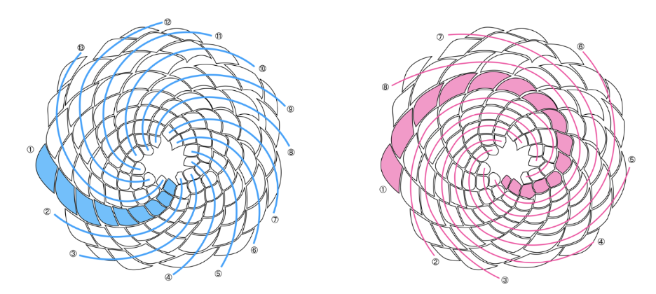
Fig. 7. Visual representation of the Fibonacci sequence in pinecones. In blue, thirteen clockwise spirals are drawn, while eight anticlockwise spirals are shown in pink (Fibonacci and pinecones, 2022).
A quantitative study by Fierz (Fierz, 2015) determined that when the number of spirals in each direction deviated from these Fibonacci numbers, the frequency of their appearance decreased as the deviation from the golden ratio increased, revealing an inversely proportional relationship between both variables. Table 1 demonstrates the various spiral patterns found in Pinus nigra cones. Upon observation, the large majority of these pinecones follow the usual 8:13 ratio between the number of clockwise and anticlockwise spirals. The ratio can be denoted as m:n in Table 1, where m and n refer to the number of spirals in the clockwise and anticlockwise directions around the pinecones. Here, m is less than n regardless of the direction of their spirals, meaning the direction of the spirals, clockwise and anticlockwise, is interchangeable so long as m is less than n (Fierz, 2015).
Table 1. Fibonacci or Fibonacci-type sequences observed in Pinus nigra cones along their deviation from the reciprocal of the golden ratio (Fierz, 2015).

Table 1 compares the spiral patterns of pinecones to the golden ratio’s reciprocal, 0.618, by calculating their respective parastichy quotients obtained by computing m/n. The deviations from 0.618 refer to how far off the pinecone’s spiral patterns are from the ideal Fibonacci spiral pattern of 8:13. As the results in Table 1 state, there is an overwhelmingly large majority of pinecones that follow the Fibonacci sequence and the golden ratio. This phenotypic expression of the spacing between pine scales is likely a result of an evolutionary adaptation requiring such structure (Okabe, 2015).
In the pinecone, the golden angle (137.5°) refers to the angle between consecutive scales (Fig. 8a) (Okabe & Yoshimura, 2021). In pinecones that do not exhibit the golden angle but rather a smaller angle between consecutive scale placements, it can be observed that the scales are much less tightly packed together as the angle decreases (Fig. 8b-c), which would expose more pine seeds before dispersal, posing a reproductive disadvantage due to the lessened protection of the samara. Therefore, the tight packing of pinecones due to the Fibonacci sequence and golden angle protects pine seeds from their exterior environment, an adaptation that increases reproductive ability (Okabe & Yoshimura, 2021).

Fig. 8. View from above of various pinecones of the Pinus thunbergii and the angles between their consecutive scales a) 137.5° b) 69° and c) 99.5° (adapted from Okabe & Yoshimura, 2021).
Environmental Modeling
Pine trees exhibit various geometric adaptations to optimize chances of survival in response to environmental factors. From changes to their height-diameter ratios to needle arrangement, pine trees architecturally adapt to survive harsh winds, temperatures, and competitive forests.
Height-Diameter Relationship
Pine tree height and diameter growth rates are influenced by a combination of genetic predisposition and morphological responses to stimuli (Opio et al., 2000). Monitoring variations in height and diameter is essential to evaluating changes in forest productivity, which plays a large role in the survival of the individual tree (Nozohourmehrabad, 2021). The height-diameter relationship (HDR) can be affected by climate, tree species, age, elevation, competition, and much more (Opio et al., 2000). Likewise, planting positions of pines and the timing of HDR measurements significantly impacts collected data (Opio et al., 2000). Such factors create varied uncertainty in HDR estimations at any given time (Zhang et al., 2014). Thus, there are many functions that model HDR, with each equation incorporating different variables to improve predictive accuracy. According to Opio and colleagues, the Weibull model (Eq. 5) was the most accurate at estimating tree height (Opio et al., 2000).

H represents the tree height in meters to the nearest tenth while D is the tree diameter in centimeters at breast height to the nearest tenth and a, b, and c are regression coefficients calculated for each species with a minimum sample of 20 trees (Height-Diameter Equations 7, 2014).
However, according to another study comparing Näslund (Eq. 6), Hossfeld (Eq. 7), Prodan (Eq. 8), and Richards’ models (Eq. 9), Hossfeld produced the best results in most of the trials (Siipilehto et al., 2023).



In the previous equation (Eq. 9), denotes breast height (Kershaw et al., n.d.)
The actual mean diameter and height points fell below the predicted values for all four of the curves (Siipilehto et al., 2023). However, the asymptotic functions, Hossfeld’s and Richards’, showed a considerably smaller inconsistency between the predicted and actual height values, as seen in Figure 9 (Siipilehto et al., 2023).

Fig. 9. Graphs of model sensitivity to varying mean height with fixed mean diameter of 24 cm for a) Näslund’s, b) Prodan’s, c) Hossfeld’s, and d) Richard’s equations (Siipilehto et al., 2023).
Table 2 displays the bias and standard deviation of prediction errors in the modelling data sets, with the best results in bold and worst results in italics (Siipilehto et al., 2023).
Table 2. Bias and standard deviation of prediction errors in the modelling data sets (Siipilehto et al., 2023)
| Model | DATA SET 1 | DATA SET 2 | DATA SET 3 | |||
|---|---|---|---|---|---|---|
| bias | s.error | bias | s.error | bias | s.error | |
| Näslund (2015) | 0.099 | 1.302 | 0.280 | 1.825 | 0.385 | 1.369 |
| Näslund | 0.051 | 1.175 | −0.159 | 1.707 | −0.272 | 1.559 |
| Hossfeld IV | −0.030 | 1.146 | −0.130 | 1.597 | −0.580 | 1.597 |
| Richards | 0.052 | 1.180 | −0.018 | 1.642 | −0.476 | 1.556 |
| Prodan | 0.055 | 1.147 | −0.102 | 1.647 | −0.241 | 1.491 |
HDR Responses to Environment
The HDR is a measure of a tree’s slenderness; thus, it can be used to assess stability. The lower the height-diameter ratio, the thicker and more stable the tree. Pines adapted to have lower H-D ratios are more equipped against wind and snow damage (Hess et al., 2020). Pines also struggle in the face of high-density forests, competing for light. In response to this environment, the trees invest more in height growth to increase sunlight exposure (Opio et al., 2000). As a result of the positive correlation between forest density and height-diameter ratio, scientists are using HDR to measure competition index for young lodgepole pines in northern British Columbia (Opio et al., 2000). Most of the models with similar climate-based parameters were found to be more accurate than the other HDR models, stressing the importance of quantifying the effect of climate change on forest structure (Nozohourmehrabad, 2021). The variables, climate moisture index and mean temperature, were linearly added to the base models to reflect the direct and indirect changes in tree height due to climate. These factors greatly influence pine tree HDR, with dry weather limiting growth to preserve water and other resources, and maximum temperature promoting growth rates. Studies show that these two variables significantly affected growth in lodgepole pines. Figure 10 displays the changing growth rate with respect to moisture index (Nozohourmehrabad, 2021).

Fig. 10. Changes in height incremental rate with respect to annual climate moisture index at given breast height for lodgepole pine (adapted from Nozohourmehrabad, 2021).
Resistance Against Strong Winds
Major mechanical injuries in trees are often the result of harsh winds with a strong lateral force of drag from the leaves (Vogel, 1996). Thus, the drag centered in the crown greatly strains the lower portions of the tree, which can potentially snap or uproot even the healthiest tree (Vogel, 1996). The applied wind and resisting forces are displayed in Figure 11. Pine trees developed a defense mechanism to combat this. A study was performed on the Maritime Pine to develop a predictive dynamic model of the mechanical response of pines to turbulent airflow (Sellier et al., 2008). Researchers concluded that the pine’s aerial architecture and turbulence structures should be further investigated as contributing factors to tree stability and wind resistance (Sellier et al., 2008). It was found that needle clustering in pines reduces aerodynamic drag by up to 40%, a storm-resisting design solution to minimize the chance of tree uprooting (Vogel, 2009). Needles within a cluster are protected from the full force of the wind by their neighboring needles. This sheltering effect reduces the drag coefficient of the entire cluster (Vogel, 2009). This drag coefficient equation is unknown due to the complexity of trees; however, researchers performed a series of calculations to estimate the drag coefficient equation of coniferous trees (Eq. 10) using data from pines in wind tunnels (Gonçalves et al., 2020).

K represents the stiffness factor, is the respective displacements, HF is the height of the load application point on the trunk, HD is the height of the trunk displacement measurement, ρ is the specific mass of the air (1.225 kg·m−3), AC is the projected crown area, HW is the height of the center of the wind pressure, and V is the wind velocity (Gonçalves et al., 2020).

Fig. 11. Applied loads and response mechanisms of tree crown’s reconfiguration ability (Gonçalves et al., 2020).
Having studied the lodgepole pine, researchers found that it had lower drag per unit of branch mass compared to other species, further supporting the importance of needle clustering (Rudnicki et al., 2004). Similarly, the clustering’s aerodynamic interference reduces convective transfer, and as a result, evaporative water loss as well, aiding the tree’s survival under droughts (Cain, 2025). Under such conditions, the number of needles per cluster can be reduced to conserve even more water (Vogel, 2009).
Probabilities and Patterns
Mathematics are also present in the growth of pine trees, whether it be their needle foliage distribution, density, or volume. Patterns can be concluded from applying various mathematical models to pine trees, notably the fractal model, to better understand their self-regulation and growth patterns.
Fractal Geometry Patterns and Resulting Benefits
Fractal geometry has often been used to describe plant structures in nature, whether it be root systems or branching patterns. Tree structures often follow two rules: firstly, crowns appear dense from a distance but less dense when viewed close up, and secondly, singular branches resemble the pattern of the entire tree (Moriguchi, 2023). These structures imply that a typical tree structure can be considered fractal, as roughly depicted in Figure 12.

Fig. 12. A fractal tree with different path developments, roughly resembling the branching pattern of a pine tree in nature (adapted from Frongillo et al., 2007).
While fractal geometry can be applied to most trees, a study on loblolly pine seedling roots attempted to quantify the less studied roots by this geometry in 1993 by Diebel & Feret. Because fractal geometry captures impressive branching patterns, it is well-suited to describing tree roots, where a well-developed root system is crucial for growth and nutriment uptake.
The Mendel’s Sponge example for fractal dimensions is used to visualize tree crowns as fractional dimensions (Mandelbrot 1983 as cited by Zeide 1998). The Mendel’s Sponge model imagines one unit cube that is divided into 27 equal cubes. With this division, each smaller cube has a side length of 1/3 . If the center cube of each face, along with the cubes behind it, are removed, only 20 cubes are left. This process is repeated, with side lengths of the smaller cubes being (1/3)2, and then (1/3)3 with each repeat. The mass decreases for each repetition, but the outer dimensions, or overall volume of the shape, remain constant. This is also applicable in two-dimensional format, as Diebel & Feret use, to analyze root structures. This is called the box-counting method. Diebel & Feret define each small two-dimensional unit square with a side of length λ, where the total number of squares Nλ. logNλ is plotted against 1/λ. The slope of this line is a fractional dimension D (Diebel & Feret, 1993).
To first determine whether the pine seedling roots were fractal and second, to determine the relationship between its fractal geometry and morphological traits, seedlings were scanned and analyzed by a computer program. The digitalized images, as shown in Figure 13, were measured using the box-counting method, dividing each image into boxes of 2 pixels by 2 pixels (Diebel & Feret, 1993).

Fig. 13. Digitized seedling root images where A is a grade 3 root, B is a grade 2 root, and C is a grade 1 root. Grade 1, 2 and 3 represents collar diameter and stem length of roots in descending order (adapted from Diebel & Feret, 1993).
The seedling roots were found to be highly fractal with fractal dimensions being highly correlated to a variety of morphological variables. These variables include projected root area, lateral or secondary branching roots dry weight, and taproot or primary root dry weight (Diebel & Feret, 1993). This branching pattern of root structures in a fractal geometry can be explained by the tree’s natural resource allocation and physiological regulation. Many growing roots arrest early or simply die due to environmental stresses such as waterlogging in spring or nutrient shortages that prevent elongation into longer roots (Wilcox, 1968). Shorter lateral roots also provide a larger surface area for nutrient uptake and turnover, allowing the tree to match seasonal pulses of resources (Wilcox, 1968). Therefore, a pine tree benefits greatly from many short lateral roots, and only a few long structural roots, naturally forming a fractal geometry in its structure.
Fractal Foliage Dispersal as Intra-Plant Competition
The traditional measurement system of length, area, or volume relies on defined objects, and is often hard to apply to organic shapes such as trees. The crown of a pine tree, for example, consists of many empty spaces between needle clusters, incomparable to the denser parts of the trunk. Fractal geometry thus also provides a solution for the volume, mass and density of these natural shapes that are neither two-dimensional surfaces nor three-dimensional solids.
The Mendel’s Sponge model presents, as detailed previously, an analogy for tree crowns, with spacing as gaps in the crown between each solid small cube as regions with foliage. When applied to actual trees, the authors adopted the method of using natural structures such as branches or shoots as each small “unit cube”. Formally, any fractal spatial dimension is defined by Equation 11:

N represents the number of smaller units, while is each unit’s side length (Zeide, 1998). The fractal spatial dimension gives information about the complexity or “space-filling” characteristics of the crown (Theiler, 1990).
Zeide uses the Mendel’s Sponge model to evaluate loblolly pine (Pinus taeda) crowns, notably the foliage dimension and the foliage density. The core principle (Eq. 12) relates the mass and density using a log-log relationship:

D represents the fractal dimension, FD is the foliage density, M is the ratio of foliage mass, V and is the volume it occupies (Zeide, 1998). This measuring model concludes that there is little correlation between fractal dimensions and variables that are indirectly related to crown size, such as age and height. The fractal dimension decreases from intermediate (trees growing under partial shade) to dominant (trees fully exposed to sunlight) trees (Zeide, 1998). These results can be interpreted as larger crowns having less dense interior foliage, with denser foliage accumulating at the periphery, a phenomenon that occurs parallel to the pine tree’s environmental situation.
The accumulation of denser foliage with leafless (or needleless, rather) foliage at the core suggests an intra-plant competition. Resources such as sunlight and nutrients are allocated carefully, and regions of branches near the periphery receive light naturally with priority. This tendency, along with apical dominance, can explain rich peripheral needle growth. A larger crown requires more resources to be allocated, resulting in a less dense foliage at the core. Nutrients, in this fashion, are prioritized to the peripheral foliage with longer lifespans (Stenberg et al., 1994).
Conclusion
From growth patterns to environmental modelling, research reveals how the pine tree embodies fundamental mathematical principles in its adaptations to ensure survival. First and foremost, the Fibonacci sequence and the golden ratio and angle found in the tree’s structure are responsible for much more than the pine tree’s beauty. The branch and needle arrangement follow the golden angle, which minimizes self-shading and maximizes light capture. These characteristics increase the trees’ chances of survival during cloudy winters. Moreover, the Fibonacci sequence and the golden angle are visibly present in pinecones, promoting a greater packing of the seeds, which increases reproductive abilities. In a similar fashion, the pine tree’s adaptive architecture has been mathematically modeled by many, uncovering the unique design solutions that make the pine so persistent. For example, in dense forests, the tree’s height-diameter ratio increases to yield tall trees with an advantage in the competition for sunlight. In stormy climates, the height growth rate decreases relative to diameter to increase stability and resistance against uprooting due to harsh winds and heavy snow. Similarly, the pine needle’s clustered arrangement also helps combat these winds by sheltering each other and ultimately reducing drag, one of the forces working against the tree. Furthermore, fractal analysis of pine tree characteristics reveals the reason for certain behaviors. The branching fractal geometry found in the pine’s roots increases resource allocation and uptake and allows for survival in nutrient shortages. Likewise, the pine’s crown foliage grows into dimensions that obey the fractal pattern, prioritizing growth in areas where sunlight and nutrients would be favored. In essence, the pine tree stands as a powerful example of how deeply mathematics is woven in nature.
References
References
Cain, J. D. (2025). Modelling Evaporation from Plant Canopies. Nerc.ac.uk. https://nora.nerc.ac.uk/id/eprint/7373/1/REPORT_NO_132_MODELLING_EVAPORATION_FROM_PLANT_CANOPIES_-_JD_CAIN.pdf
Chourasia, M. (2025). The Golden Angle? Medium. https://medium.com/beyond-the-symbols/the-golden-angle-04b36892fd93
Chowdary, P. S. R., Prasad, A. M., Rao, P. M., & Anguera, J. (2015). Design and Performance Study of Sierpinski Fractal Based Patch Antennas for Multiband and Miniaturization Characteristics. Wireless Personal Communications, 83(3), 1713-1730. https://doi.org/10.1007/s11277-015-2472-5
Diebel, K. E., & Feret, P. P. (1993). Using Fractal Geometry to Quantify Loblolly Pine Seedling
Root System Architecture. Southern Journal of Applied Forestry, 17(3), 130-134. https://doi.org/10.1093/sjaf/17.3.130
Fibonacci and Golden Ratio. (2023). Let’s Talk Science. https://letstalkscience.ca/educational-resources/backgrounders/fibonacci-and-golden-ratio
Fibonacci and pinecones. (2022). The Craft of Coding. https://craftofcoding.wordpress.com/2022/05/11/fibonacci-and-pinecones/
Fierz, V. (2015). Aberrant phyllotactic patterns in cones of some conifers: a quantitative study. Acta Societatis Botanicorum Poloniae, 84(2), 261–265. https://doi.org/10.5586/asbp.2015.025
Frongillo, R. M., Lock, E., & Brown, D. A. (2007). Symmetric fractal trees in three dimensions.
Chaos, Solitons & Fractals, 32(2), 284-295. https://doi.org/10.1016/j.chaos.2006.04.036
Gonçalves, R., Linhares, C., & Yojo, T. (2020). Drag coefficient in urban trees. Trees. https://doi.org/10.1007/s00468-019-01951-1
Height-Diameter Equations 7. (2014). https://www2.gov.bc.ca/assets/gov/farming-natural-resources-and-industry/forestry/timber-pricing/timber-cruising/cruise-compilation-manual/cruise_comp_ch7.pdf
Hess, A. F., Minatti, M., Costa, E. A., Schorr, L. P. B., da Rosa, G. T., de Arruda Souza, I., Borsoi, G. A., Liesenberg, V., Stepka, T. F., & Abatti, R. (2020). Height-to-diameter ratios with temporal and dendro/morphometric variables for Brazilian pine in south Brazil. Journal of Forestry Research, 32(1), 191–202. https://doi.org/10.1007/s11676-019-01084-8
Humaira. (2023). Unraveling the Magic: A Fibonacci Sequence Day Celebration for Math Enthusiasts [Webpage]. https://medium.com/@humab9382/unraveling-the-magic-a-fibonacci-sequence-day-celebration-for-math-enthusiasts-99b0af2f41c7
Kershaw, J., Morrissey, R., Jacobs, D., Seifert, J., & Mccarter, J. (n.d.). DOMINANT HEIGHT-BASED HEIGHT-DIAMETER EQUATIONS FOR TREES IN SOUTHERN INDIANA. Retrieved November 7, 2025, from https://www.nrs.fs.usda.gov/pubs/gtr/gtr-p-24%20papers/39kershaw-p-24.pdf
King, S., Beck, F., & Lüttge, U. (2004). On the mystery of the golden angle in phyllotaxis. Plant Cell & Environment, 27(6), 685-695. https://doi.org/10.1111/j.1365-3040.2004.01185.x
Moriguchi, K. (2023). Estimation of fractal dimension of trees using LiDAR point data with
sequential data decimation. Remote Sensing of Environment, 295, 113722. https://doi.org/10.1016/j.rse.2023.113722
Nozohourmehrabad, P. (2021). Modelling Tree Height-Diameter Relationships and the Effect of Climate. University of Alberta Library. https://doi.org/10.7939/r3-sgx1-6e67
Opio, C., Jacob, N., & Coopersmith, D. (2000). Height to diameter ratio as a competition index for young conifer plantations in northern British Columbia, Canada. Forest Ecology and Management, 137(1-3), 245–252. https://doi.org/10.1016/s0378-1127(99)00312-6
Okabe, T. (2015). Biophysical optimality of the golden angle in phyllotaxis. Scientific Reports, 5(1). https://doi.org/10.1038/srep15358
Okabe, T., & Yoshimura, J. (2021). Two-step mechanism of spiral phyllotaxis. Journal of Theoretical Biology, 508, 110484. https://doi.org/10.1016/j.jtbi.2020.110484
Pierce, R. (2025). Fibonacci Sequence. https://www.mathsisfun.com/numbers/fibonacci-sequence.html
Pine Cones and the Fibonacci Sequence. (2019). Awkward Botany. https://awkwardbotany.com/2019/12/25/pine-cones-and-the-fibonacci-sequence/#:~:text=The%20pattern%20of%20spirals%20on%20pine%20cones,Artichokes%20*%20Cauliflower%20florets%20*%20Leaf%20arrangements
Pine Tree Number Patterns. Texas Parks & Wildlife. https://tpwd.texas.gov/education/resources/resources/lesson-plans/texas-regions/pineywoods/pine-tree-number-patterns#:~:text=Background,following%20the%20following%20number%20patterns
Pont, D. (2001). Use of Phyllotaxis To Predict Arrangement and Size of Branches in Pinus radiata. New Zealand Journal of Forestry Science 31(2), 247-262.
Rudnicki, M., Mitchell, S. J., & Novak, M. D. (2004). Wind tunnel measurements of crown streamlining and drag relationships for three conifer species. Canadian Journal of Forest Research, 34(3), 666–676. https://doi.org/10.1139/x03-233
Sellier, D., Brunet, Y., & Fourcaud, T. (2008). A numerical model of tree aerodynamic response to a turbulent airflow. Forestry, 81(3), 279–297. https://doi.org/10.1093/forestry/cpn024
Siipilehto, J., Sarkkola, S., Nuutinen, Y., & Mehtätalo, L. (2023). Predicting height-diameter relationship in uneven-aged stands in Finland. Forest Ecology and Management, 549, 121486–121486. https://doi.org/10.1016/j.foreco.2023.121486
Shamsheer. (2020). 5 Mathematical Patterns in Nature: Fibonacci, Fractals and More
[Webpage]. https://owlcation.com/stem/astounding-ways-how-mathematics-is-a- part-of-nature-
Singh, S. P., Inderjit, Singh, J. S., Majumdar, S., Moyano, J., Nuñez, M. A., & Richardson, D. M.
(2018). Insights on the persistence of pines (<i>Pinus</i>species) in the Late Cretaceous and their increasing dominance in the Anthropocene. Ecology and Evolution, 8(20), 10345-10359. https://doi.org/10.1002/ece3.4499
Stenberg, P., Kuuluvainen, T., Kellomäki, S., Grace, J. C., Jokela, E. J., & Gholz, H. L. (1994).
Crown Structure, Light Interception and Productivity of Pine Trees and Stands.
Ecological Bulletins, 43, 20–34. http://www.jstor.org/stable/20113129
Theiler, J. (1990). Estimating fractal dimension. Journal of the Optical Society of America A,
7(6), 1055. https://doi.org/10.1364/josaa.7.001055
Vogel, S. (1996). Blowing in the Wind: Storm-Resisting Features of the Design of Trees. Arboriculture & Urban Forestry, 22(2), 92–98. https://doi.org/10.48044/jauf.1996.013
Vogel, S. (2009). Leaves in the lowest and highest winds: temperature, force and shape. New Phytologist, 183(1), 13–26. https://doi.org/10.1111/j.1469-8137.2009.02854.x
Wilcox, H. E. (1968). MORPHOLOGICAL STUDIES OF THE ROOT OF RED PINE, PINUS
RESINOSA I. GROWTH CHARACTERISTICS AND PATTERNS OF BRANCHING. American
Journal of Botany, 55(2), 247-254. https://doi.org/10.1002/j.1537-
2197.1968.tb06968.x
Zeide, B. (1998). Fractal analysis of foliage distribution in loblolly pine crowns. Canadian
Journal of Forest Research, 28(1), 106-114. https://doi.org/10.1139/x97-202
Zeng, L., & Wang, G. (2009). Modeling golden section in plants. Progress in Natural Science, 19(2), 255-260. https://doi.org/https://doi.org/10.1016/j.pnsc.2008.07.004
Zhang, X., Duan, A., Zhang, J., & Xiang, C. (2014). Estimating Tree Height-Diameter Models with the Bayesian Method. The Scientific World Journal, 2014, 1–9. https://doi.org/10.1155/2014/683691
- The divergence angle corresponds to the angle between successive branches or between successive needle clusters.