
Table of Contents
On this page
- Abstract
- Introduction
- Scaling and Territory Size in Limpets
- Self-thinning in Barnacles and Geometry of Packing
- Barnacle Shell Dimorphism and Evolutionary Game Theory
- A Mathematical Model for Barnacle Shell Dimorphism
- Modelling Limpet Populations
- Motility Patterns in Limpets
- Crisp’s Behavioural Model
- Conclusion
- References
Keywords: Barnacles, limpets, mathematical patterns, modelling, game theory, and evolutionary pressure.
Abstract
The mathematical properties and patterns underlying barnacles and limpets’ adaptations are analyzed in this paper. Many biological quantities can be expressed as power functions that vary with respect to the organism's body mass. For example, in the limpet Lottia gigantea, studies have shown that an individual's territory size is proportional to the square root of its shell length—an ecological factor that influences interactions with neighboring organisms.
The paper also explores how limpet populations can be modeled using State-and-Prediction-Based Theory (SPT), which accounts for adaptive behaviors in dynamic environments. Limpet motility, shaped by a range of evolutionary pressures, follows complex patterns that can be studied mathematically.
Finally, Crisp’s model is discussed as a framework for understanding cyprid larval behavior during settlement. The model highlights how cyprids actively evaluate surfaces using biological and physical cues, influencing adult barnacle distribution.
Overall, this analysis demonstrates how mathematical principles can illuminate fundamental aspects of adaptation in barnacles and limpets.
Introduction
Barnacles and limpets are unique superorganisms that inhabit the intertidal zone, characterized by rocky shores, varying tides and a turbulent environment (Adey & Loveland, 2007), which gives way to evolutionary traits that are quite distinct from other marine animals. Being mostly sessile, they aggregate in large colonies along the rocky shores (see below) and interact in a fascinating way with one another and with other neighbouring species.

Fig. 1. A large colony of barnacles (left) and limpets (right). Adapted from (Denny & Gaines, 2007; US National Oceanic and Atmospheric Administration, n.d.).
What laws then govern the expression of these unique evolutionary traits? How can the interactions between individuals and populations be modelled and analyzed? This paper will present an overview of the mathematical principles and theories that can be used to describe the design solutions and superorganism behaviour of barnacles and limpets. It will begin by discussing scaling laws as they apply to territory size and shell packing, followed by an investigation into evolutionary game theory and population dynamics. Finally, a discussion on motility patterns and settlement dynamics will conclude the mathematical analysis.
Scaling and Territory Size in Limpets
Many biological quantities vary as a function of body mass and can be described by a power law of the form:

where f is the biological quantity in question, M is the body mass, b is the scaling exponent and a is a constant (Denny & Gaines, 2007). When b = 1, the quantity f grows linearly as a function of mass, and we say that the relationship is isometric. In many cases, however, b ≠ 1, where one quantity grows faster than the other and the relationship is called allometric.
This is the case for the area of the home range of an organism, for example, in the case of terrestrial mammals, as the animals grow larger, their demand for resources to fuel their metabolic needs also grows. Larger animals within a colony must compete for more resources with their neighbours as both require more nutrients to sustain their metabolic demands. It is expected, then, that the home range of these animals grows faster than the size of the animals which occupy it, and thus the scaling exponent b > 1 (Denny & Gaines, 2007).
Unlike land animals, there have been few documented cases of this territorial behaviour in invertebrates, and this widely accepted model for territorial behaviour is more difficult to apply to limpets because they are mainly sessile. The territory, or home range of limpets, is thus restricted to the spot in which they settle and the small area around it that is easily accessible to them. Unlike terrestrial mammals, which defend an exponentially larger territory as their body size grows larger (b > 1), the owl limpet Lottia Gigantea has been found to exhibit the opposite behaviour, as seen in Fig. 2 below. Indeed, the square root of the area of the home range increases linearly with shell size, indicating slower growth relative to body size (b < 1) (Stimson, 1970).

Fig. 2. Relationship between shell length and area of the home range for the limpet Lottia Gigantea (Stimson, 1970).
For this to occur, there must be some way that limpets are able to guard their territory and reduce competition for resources. Indeed, Lottia exhibits distinct behaviours in response to different types of intruders. When encountering predatory snails such as Thais Emarginata and Acanthina pirata, its reaction mirrors that observed with Acmaea, but considerably faster, as seen in Table 1. However, its behaviour can vary. In some cases, Lottia lifts its shell and forcefully brings it down onto the anterior edge of the snail's foot, which makes the predator retract, lose its hold, and get carried away by the water (Stimson, 1970).
Table 1. Lottia's reaction times to several intertidal snail species (Stimson, 1970).
| Species | Number of trials | Reaction time (sec) | Welch's "t" statistic | Significance level, P |
|---|---|---|---|---|
| Thais emarginata | 14 | 16.6 ± 10.0 |
4.27 |
< 0.01 |
| Tegula funebralis | 14 | 43 ± 20.9 | ||
| Acmaea | ||||
(several species) | 23 | 34.0 ± 20.7 | ||
Additionally, these limpets interact with sedentary organisms such as anemones, barnacles, and mussels. While barnacles typically mark the limpet’s territory, they can occasionally be found within it, particularly in cracks or pits. Evidence from their excrement, which contains barnacle exoskeletons, suggests that tiny, recently settled barnacles are scraped off during grazing. These observations highlight the adaptive responses of the limpet to different intruders in its habitat (Stimson, 1970).
Research conducted in Scotland has shown that by physically scraping or rasping newly settled barnacles (Balanus balanoides) off the substrate, Patella vulgata, another giant limpet, may dramatically lower their density.
Similarly, Lottia eradicated one-third of the barnacles in a month after being introduced to an area where small Chthamalus fissus (3 mm in basal diameter) were present, eventually bringing their numbers down to less than 20%. This removal likely occurred through a combination of rasping and dislodging. In contrast, barnacles in a nearby area that Lottia could not access remained unaffected, indicating the direct influence of Lottia’s grazing on barnacle density (Stimson, 1970).
It seems that Lottia responds selectively to intruding items. When presented with steel pegs, pencil erasers, or even a human finger held in front of them for two minutes—an ample amount of time for them to react to typical grazers or predators—Lottia showed no response (Stimson, 1970).
Ultimately, Lottia's responses to intruders fall into three distinct categories: predators, competitors for space, and competitors for food. The various responses to predators and grazers, as well as the absence of sensitivity to inanimate foreign items, indicate that Lottia can distinguish between different kinds of intruders (Stimson, 1970).
Rather than treating all objects as mere obstructions, Lottia appears to evaluate the nature of each intruder and react appropriately, exhibiting a sophisticated territorial defence strategy.
Self-thinning in Barnacles and Geometry of Packing
As sessile marine creatures, barnacles have difficulties in their crowded intertidal habitats (shown in Fig. 3). As barnacle populations grow, individuals compete not only for space but also for access to nutrients and sunlight. To address the difficulties caused by high population density and limited resources, these creatures use self-thinning as a natural regulating mechanism.

Fig. 3. Densely packed colony of Barnacles (Lisa, n.d.).
Self-thinning is known as the decrease in population density brought on by competitively induced losses within a cohort of organisms that are growing. In fact, weaker or smaller individuals are selectively killed out because of competition for limited resources like nutrients, light, or space. As they have greater access to resources, the surviving organisms get bigger over time, which lowers population density but increases individual biomass.
The negative-power function of individual mass on population density is the outcome of the survivors' continuous growth. For barnacles, the exponent of this function reflects the relationship between their population density and individual size, driven by competition for space and resources. The exponent of this function tends toward -3/2 among plants, indicating a relationship between the area occupied and the individual volume or mass and highlighting a universal scaling law in self-thinning processes across different species.
The power equation M = kDa of the same form as Equation (1), where a=-3/2, establishes a relationship between the population density (D) and the mean individual mass of survivors (M) (Sibomana et al., 2013).
On the assumption of isometric growth, a basic geometric model of self-thinning has been developed. Therefore, the area occupied per individual (A) must be inversely proportional to population density (N) when space is fully utilized and surviving individuals continue to grow (Hughes & Griffiths, 1988).
Semibalanus balanoides, one of the barnacle populations in the Menai straits, are impacted by an annual recruitment process that saturates cleared substrata after older cohorts are dislodged during severe weather. Because of this colonization cycle, adjacent substratum patches are frequently occupied by variously aged cohorts, each of which has unique mean barnacle sizes and population densities. The body dimensions and mass of barnacles from single-cohort areas were measured. The relationship between individual mass (W) and rostro-carinal diameter (L) follows an allometric scaling law, with an exponent of 3.7. Similarly, mass was related to basal area (A) with an exponent of 2.2. As seen in Fig. 4, to assess population characteristics on a broader scale, mass per unit area (B) was regressed against population density (N), revealing patterns in resource distribution and growth constraints. The slope of -0.68 aligns closely with the value predicted from growth allometries (1−3.7/2.2) (Sibomana et al., 2013).

Fig. 4. Double-logarithmic plot of mass per unit of area (B) on population density (N) for Semibalanus balanoides (Sibomana et al., 2013).
Substantial shape changes impact allometric growth of barnacles, which is fueled by the extreme restriction on lateral expansion in densely packed populations.
In fact, the truncated conical shape of uncrowded barnacles is characterized by a base diameter that is greater than its height. Growth is gradually restricted to the vertical plane by crowding. Height first equals, then surpasses, the basal diameter. The shape quickly changes from a truncated cone to a cylinder (as seen in Fig. 5) and then to a flared cylinder with the apical diameter greater than the basal diameter (Sibomana et al., 2013).

Fig. 5. Geometric Volume Transformations: (a) Truncated Cone to (b) Regular Cylinder (Cheng et al., 2014).
This latter phenomenon is significant due to the relatively small area of attachment needed to anchor densely packed individuals and the necessity of maintaining a proper ratio between body mass and trophic apparatus size (proportional to the rostro-carinal diameter). As seen in Fig. 6, height is proportional to the square of the rostro-carinal diameter, measured across a broad range of population densities, due to the shape change (Sibomana et al., 2013).

Fig. 6. Double-logarithmic plot of individual height (H) on rostro-carinal diameter (L) for Semibalanus balanoides (Sibomana et al., 2013).
Because the rostro-carinal diameter grows more quickly than the basal diameter, barnacle groups generate hummocks, which lose mechanical stability as they become more pronounced. Eventually, these hummocks may be dislodged from the substratum by powerful tidal current surges. In contrast, the self-thinning process, which begins prior to hummock formation, does not result in such mass mortality.
Moreover, self-thinning results from the death of individuals undercut and laterally displaced by more vigorous neighbors. However, size of barnacles is not highly associated with future competitive success, unlike certain plant communities where dominant individuals consistently inhibit the growth of inferior neighbors. Individuals may be able to leapfrog one another due to unpredictable suppression or elevation of growth, possibly caused by randomly varying feeding success. Therefore, even though the proximal mechanism of competition in barnacles is lateral compression, the victims are not always the ones that are originally weaker (Sibomana et al., 2013).
Recounting what has been said, density-dependent disappearance (self-thinning) occurs in tandem with individual growth within barnacle cohorts, with the result that, over the course of time, mean individual mass is related to population density by an exponent of approximately -3/2. This value is set by the geometry of packing on the substratum. For populations that have not reached asymptotic biomass, allometric growth and multilayered packing provide a sufficient explanation for the observed deviations from -3/2 (Sibomana et al., 2013).
Barnacle Shell Dimorphism and Evolutionary Game Theory
In the Physics paper, it was discussed that the barnacle species Chthamalus anisopoma, native to the northern Gulf of California, is dimorphic in shell morphology. Recall that this species shares a habitat with a specialized predator, Acanthina angelica, which attacks the barnacles through the opercular plate. C. anisopoma has developed a unique defence mechanism to counter this attack by rotating the operculum 90° (see Fig. 7), but this defence comes at a cost: the defended form grows more slowly and makes the barnacles less fecund (Lively, 2021). As such, not all individuals adopt the defended form, and we can mathematically model this evolutionary trait to better understand this design solution.
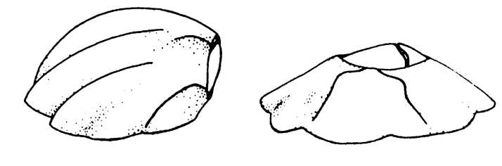
Fig. 7. Comparison of defended (left) and undefended (right) shell morphologies (Lively, 2021).
The mathematical model that describes the proportion of the barnacle population which adopts either morphology is based on evolutionary game theory. Game theory is a branch of mathematics that addresses situations in which an individual must make a decision, and the result of their decision depends not only on them, but also on the decisions of those around them (Easley & Kleinberg, 2010). In evolutionary game theory, we say that a strategy—that is, a set of actions that an individual elects to take—is evolutionarily stable if it is a strategy that tends to persist in time, driving the population into an equilibrium known as the evolutionarily stable state. If a strategy remains evolutionarily stable, then any other intruding set of individuals who adopt a different strategy will be weaker and die off over time (Easley & Kleinberg, 2010).
More formally, consider two strategies within a population: a dominant one, denoted D, and an invasive one, denoted I. We say that the fitness k of a particular morph (i.e., a group of individuals adopting the same strategy) measures that morph’s ability to thrive in the population by feeding and reproducing. Higher fitness results in a higher probability of reproductive success, thus creating more offspring with the same evolutionary strategy. The dominant strategy D is evolutionarily stable if members adopting that strategy have strictly greater fitness than those adopting the invasive strategy I. Namely,

where kD and kI are the fitness levels of each morph (Easley & Kleinberg, 2010).
In many cases, however, it’s not as simple as saying that one single strategy is evolutionarily stable and dominates all others. This is the case for C. anisopoma, where the evolutionarily stable state is said to be mixed—that is, two or more distinct strategies exist within the population, and the proportion of the population which adopts each strategy remains relatively constant in time (Lively, 2021). Increased complexity of the organism and the ecosystem results in a more elaborate mathematical model, giving rise to such mixed states.
To avoid desiccation, the predatory snail A. angelica tends to move into rock crevices as the tide falls. As such, the predation risk is higher around these crevices and lower further away (Lively, 2021). It is thus believed that the location in which the barnacle cyprids settle influences the strategy that they will adopt. As such, the mathematical model considers both the cost of inducibility—namely, the loss of fitness in individuals that adopt the defended morphology—and spatial correlation, as it is assumed that neighbouring barnacles will adopt a similar strategy due to similar predation risk.
A Mathematical Model for Barnacle Shell Dimorphism
Let the probability of a cyprid settling in a low-predation area be ρ. It follows that the probability of settling in a high-predation area is 1 - ρ. Let the fitness of defended individuals be kD, and let eDU be the relative fitness of a defended individual in a population composed mainly of the undefended morph. Notice, in this case, that the defended strategy is considered invasive (I). Similarly, eUD is the relative fitness of an undefended individual within an overall defended population. It is assumed that it is difficult for an undefended individual to survive in a high-predation area because they will fall prey too easily to A. angelica. On the other hand, defended individuals have a difficult time surviving in a low-predation area because they have a lower relative fitness.
The absolute individual fitness of an individual, considering the location in which it settles, the strategy it adopts, and the relative fitness of that strategy versus the rest of the population, is given by:

where Wi is the absolute individual fitness, q is the probability that all individuals adopt the undefended form, and qi is the probability that the particular individual will adopt the undefended form (Lively, 2021).
This equation is extremely complicated to understand, but what is important to note are the parameters that govern the overall fitness of an individual. Recall that higher fitness results in higher reproductive success for that individual. From Equation (3), it can be found that a mixture of both defended and undefended individuals occurs when

and thus, the population will be composed purely of the defended morph for p < (keDD) / eUD, and entirely of the undefended morph for p > k / (eUU + k(1 - eDU)) (Lively, 2021). The values of the constants ρ, k, q, and eij can be obtained experimentally by conducting research in the field (Orr, 2009).
Modelling Limpet Populations
What is the state—and predictive—based theory?
In the modern theory of ecology, it is highlighted how individual organism behaviors act in a way to maximize a particular measure of fitness at a future time. Recall that a measure of fitness can be described as anything the organism is aiming for, such as the search for food, the need to avoid predators, or the storing of energy for reproduction. When the current state of the organism is taken into consideration—most often its energy reserves, the model becomes state-dependent. For example, a hungry animal will take greater risks to search for food compared to a satiated one (Railsback et al., 2020).
Individual-based models (IBMs) solely focus on individuals for the modelling of population. This independence from more system-level theories facilitates the modelling of the effects of adapting behaviors. In IBMs of adaptive individuals, the system dynamic emerges from the interdependence of each organism and their trade-offs for different measures of fitness. However, including adaptive behaviors in IBMs can be a tedious task, and many ways have been proposed to solve this problem. For instance, dynamic state variable modelling (DVSM) is a method used where an individual optimal measure of fitness is defined at a future time, and a dynamic optimization program finds the necessary behaviors needed to achieve it. However, such method has shown to be problematic with the parallel use of IBMs, as DVSM often need knowledge inaccessible for individual organisms, such as predator avoidance habitats or the presence of food in certain areas (Railsback et al., 2020).
Railsback et al., showed how ecology did not have proper theories that could be used for predicting the population dynamics of organisms that show adaptive trade-off behaviors (Railsback et al., 2020). Thus, they formulated the state—and predictive—based theory (SPT), which comes in place to mitigate the problems that arise with the use of IBMs and DVSMs. Hence, they build this new model with the following characteristics:
- Individuals in the population are unique (such as in size, life stage, social status or energy reserves).
- Individuals must go through a life cycle, and much change during that time.
- Individuals interact with their environment and other individuals, which can affect—on a local level—their behavior’s success.
- Individuals’ interactions with others induce behavioral feedback, which affects how the individual behaves.
- The environment changes spatially, and most of it provides high risks to the organism (non-favorable for feeding).
- The environment changes over time.
(Railsback et al., 2020)
SPT uses these complexities as roots during the optimization process. Much like DVSM, SPT will consider a favorable measure of fitness in the future and will seek the most probable sequence of behavioral trade-off needed for an individual to reach this fitness. However, unlike DVSM which utilizes a one-time optimization of an individual behavior for the entire simulation, SPT updates the individual’s behavior at consistent time steps. This allows for the sought adaptive behavior trade-offs, where the individual will update their decisions based on their internal and external state (Railsback et al., 2020).
How is SPT applied to limpet populations?
Limpets forage for food on the sea floors of intertidal zones. They prefer to stay in the wave splash during feeding, as it protects them from predator attacks and desiccation. Periods of low and high tides often show greater risks for their survival. Therefore, they move up the shore and rest until conditions become favorable for feeding. However, they sometimes stay in the wave zone, instead of expending the energy needed to reach the rest zone. Hence, we can see how limpets’ foraging behavior consist of feeding as much as possible during favorable times, while deciding whether to assume the energy cost of moving to the rest place during unfavorable feeding times (Railsback et al., 2020).
By basing their model on these descriptions, Railsback and colleagues were able to conceive a model with the following characteristics:
- Given HA is the mean number of hours limpets pass in the wave zone, and HF is the mean number of hours they pass in the favorable tidal zone for feeding. Then the following were observed in the limpet Cella grata:
- If HF was less than five hours, then HA was equal or greater than HF.
- If HF was between five and 15 hours, then limpets would forage for most of the time.
- If HF was greater than 15 hours, there would not be an increase in activity with the additional hours of favorable conditions.
- The definition of the following variables:
- favorable? which defines whether the environment favors feeding or not.
- The time (from 0 to 23.5 hours).
- w, which defines its energy reserves (in J).
- g, which defines the gut content of the limpet (in mm3). This represents the volume of food which has been eaten, but not yet digested by the limpet, which means that this does not contribute to the energy reserves.
- activity, which describes the state of limpet. This variable can take the values of feeding, stasis (when the limpet is not feeding but staying in the wave zone), and resting (when the limpet has moved from the wave zone to the rest zone).
- The time-steps—when the behavior of the limpets is updated—are 0.5 hours.
At the start of the simulation (at time zero), the variable favorable? is set to true, activity is set to “resting”, the energy reserves w is set to maximum (wmax), and the gut contents g is set to zero (Railsback et al., 2020).
During the simulation, the energy balance is updated at every time-step with the following equation:

where wt depicts the energy reserve (J) for the current time-step, C is the energy cost (J) for the time-step, δ is the energy content of food (1.66 J/ mm3), and σ is the volume (mm3) of the food which is processed into energy (Railsback et al., 2020).
The variable C, the energy cost, consists of the respiration and the production of mucus during the displacement of a limpet. The model defines the following constant values for C.
- If activity is “resting” and was “resting” in the previous time-step, then C is equal to 6.23 J.
- If activity is “resting” and was “stasis” or “feeding” in the previous time-step, then C is equal to 135.7 J (as the limpet must have moved to the resting zone).
- If activity is “feeding”, then C is equal to 49.4 J.
- If activity is “stasis”, then C is equal to 6.23 J.
(Railsback et al., 2020).
The gut content, g, will affect the volume of the food processed into energy, σ. Indeed, if the total volume of food in the guts of the limpet is greater than the amount of food that can be processed per time-step, then σ takes the value of this maximum (σmax = 23.6 mm3). Otherwise, σ will take the value of gt-1 (Railsback et al., 2020).
Based on this, g is updated according to the following equation:

where λ is the food ingestion rate (of 70.7 mm3 per time step when activity is set to “feeding”), and gmax is the maximum gut content, which is of 207 mm3 (Railsback et al., 2020).
Results from the application of the SPT to predict foraging behaviour of Cella grata
In this model, reproduction is not considered. Therefore, we only consider two adaptive foraging decisions: energy intake and reserves, or protection against predators and desiccation. The length of the simulation is one day, which allows for a full cycle of favorable and unfavorable feeding conditions. Furthermore, the fitness measure is the mean energy reserves throughout the day. Predicting the activity of the limpet is also crucial. It is not possible to only set one variable for activity and hope to optimize the simulation, as it would starve even when feeding (as it loses energy while feeding). Therefore, the model programs the limpet to alternate between feeding and stasis during favorable time-steps, while resting during all unfavorable time-steps. This allows for the limpet to feed only, when necessary, while relying on resting or stasis if it sill maximizes the mean energy reserves for the rest of the day (Railsback et al., 2020).
The result of the simulation can be seen in Fig. 8.

Fig. 8. Simulation result of the application of SPT on a limpet for the first two days and with 10 favorable hours per day. The solid lines represent the energy reserves, and the dashed lines represent the gut content at the end of each time-step. The open-circle depicts feeding, the X depicts stasis, and the solid black bars represent resting (Railsback et al., 2020).
This plot does show the basic patterns observed in limpet behaviors. Indeed, it is shown how limpets alternate between feeding and stasis during favorable periods, and how they fill their gut content before unfavorable periods. Furthermore, energy reserve dip during extensive feeding to refill the limpet’s guts, and during the start of the unfavorable periods, because of the cost of moving from the wave zone to the rest zone (Railsback et al., 2020). Hence, we see how SPT can successfully predict behaviours of adaptive individuals such as limpets.
Motility Patterns in Limpets
Although exhibiting slow and little movement, limpets demonstrate remarkable activity rhythms and behaviours which are primary adaptations to environmental stresses. For example, the species Siphonaria capensis present intricate motility patterns, depending on tide levels, limpets’ dwelling, and time of day. When analyzed from a homing point of view, this species of limpets may be divided into two types: pool-dwelling limpets and dry-rock limpets. Regardless of their position, these limpets demonstrate an increase in activity during low tides, minimizing the risk of dislodgement off the substrate by waves. However, a notable difference between pool-dwelling and dry-rock limpets is the time of their activity. Pool-dwelling limpets express no preference regarding the time of day, as they move during day and night. On the other hand, dry-rock limpets showed a preference of moving only at night. The latter difference can be observed in Fig. 9. (Branch & Cherry, 1985).

Fig. 9. Activity rhythms of Siphonaria capensis. A) pool-dwelling limpets. B) dry-rock limpets (Branch & Cherry, 1985).
Homing Mechanism
The reason behind the restricted movement of dry-rock limpets is the avoidance of desiccation. When moving, limpets are prone to losing body water and moisture, especially during the day. When limpets stay on their home scar, they create a tight seal which allows them to maintain their water reservoir, minimizing desiccation (Branch & Cherry, 1985).
When limpets settle, they choose a home and form a home scar. The home scar is formed due to mechanical pressure from the limpets’ shell on the substate, and it provides a tight seal between the shell and the substrate due to a perfect fit between the two. However far limpets travel, they almost always return home, demonstrating remarkable fidelity to their homes. As mentioned, home scars reduce water loss in dry-rock limpets, minimizing the risk of desiccation. For pool-dwelling limpets, the risk of desiccation is already minimal due to their habitat, yet they still exhibit a remarkable homing behaviour. It has been found that homing scars help reduce osmotic stress with fluctuating salinities, which describes the amount of salt found in water at a given time, due to evaporation or rainfall. Fig. 10 shows the osmotic concentration of pool-dwelling limpets in low versus high salinity environments. Limpets that were undisturbed and remained on their home scar resisted changes in their osmotic concentration, whereas limpets that were moved away from their home scar exhibited significant fluctuations (Branch & Cherry, 1985).

Fig. 10. The osmotic concentration of pool-dwelling limpets left undisturbed on their home scars, lifted and replaced on scars (disturbed), or denied access to their scars in (A) hyposaline environments and (B) hypersaline environments (Branch & Cherry, 1985).
Crisp’s Behavioural Model
In their larval stage, barnacles have intricate settling behaviours that were initially described by Prof. Dennis Crisp. Specifically, the cyprid stage is the larval stage which is responsible for searching and settling on a suitable substrate. Crisp’s model divides the process of barnacle cyprid settlement into three phases: wide searching, close searching, and inspection. Wide searching describes the cyprid exploring large areas to identify potential settlement locations, with constant movement of their appendages. Close searching describes the concentration on a smaller area, with a higher frequency in appendage movement, representing linear increase. Lastly, inspection describes the phase when the cyprid attaches temporarily to the substrate and probes the local surface’s characteristics, using its appendages, before permanent cementation (Crisp et al., 2013).
A study done by Aldred et al. confirmed the validity of Crisp’s behavioural model. The study uses an advanced novel tracking technology that allowed for the analysis of cyprids’ body movement. Using this quantitative model for cyprids’ body movement, the three phases of settlement were observed. Fig. 11 is a representation of the data obtained in study. The graph demonstrates the number of movements per appendage as a function of time until the cyprid settles permanently. In addition, the state of the cyprid was documented to keep track whether the cyprid is temporarily anchored or moving freely, as in walking. Phase (i) represents zero or minimal increase in the number of movements with time, but the cyprid was walking, indicating the first stage which is wide searching. Phase (ii) represents zero or minimal increase min the number of movements with time as well, but the cyprid is not walking, indicating a non-exploratory phase. Phase (iii) exhibits a linear increase of body movements with time, accompanied by walking, indicating the second stage which is close searching. Finally, phase (iv) demonstrates a linear increase of body movements with time, but the cyprid is temporarily anchored, which represents the third stage in Crisp’s model, inspection (Aldred et al., 2018).

Fig. 11. Tracking plot of a single cyprid divided into different phases, using movement of cyprid’s body as a function of time in hours. (i) represents wide searching phase. (ii) represents a non-exploratory phase. (iii) represents close searching phase. (iv) represents inspection behaviour (Aldred et al., 2018).
Conclusion
From a mathematical and modelling perspective, limpets and barnacles exhibit fascinating design solutions which help them survive in their severe environments. Limpets, for example, exhibit an intricate motility pattern, which helps them optimize environmental stresses. Due to their habitat, limpets are susceptible to desiccation from the sun or fluctuation in their osmotic concentrations due to salinity changes in the water. To alleviate these stresses, limpets exhibit a loyal homing mechanism, where they always return to their home scar. At the home scar, limpets can mitigate water loss and osmotic stress due to the tight seal that is formed between the limpet shell and the substrate.
Barnacles, on the other hand, exhibit a unique adaptive morphology to withstand environmental stresses. The snail Acanthina angelica poses a serious threat to the barnacle Chthamalus anisopoma, which lives in intertidal zones that are rich in predators. Some individuals rotate their operculum 90 degrees in a unique shell form to protect themselves from predators. In spite the fact that this change reduces susceptibility, it also slows growth and decreases fertility. Barnacles maximize their survival in changeable situations by balancing their defended and undefended morphologies.
Moreover, one challenge barnacles face is the high competition for space and resources in crowded intertidal zones. The solution is self-thinning in barnacle populations which mitigates the effects of overcrowding by balancing individual growth and density through allometric scaling and geometric adaptations. These mechanisms enable barnacles to optimize resource use and maintain population stability in their environment.
In their intertidal environment, limpets must balance avoiding predators and consuming energy. By switching between feeding, stasis, and resting, limpets maximize their foraging behavior according to the state-and predictive-based theory (SPT). With this adaptive technique, they can exhibit a well-balanced trade-off between survival and resource acquisition, maximizing energy reserves at favorable times and limiting dangers and energy consumption during unfavorable ones.
Indeed, limpets and barnacles demonstrate how remarkably adept nature is at adjusting to harsh conditions. By examining their distinct characteristics, we can identify strategies that could result in ground-breaking engineering breakthroughs.
References
References
Adey, W. H., & Loveland, K. (2007). CHAPTER 2 - The Envelope: Physical Parameters and Energy State. In W. H. Adey & K. Loveland (Eds.), Dynamic Aquaria (Third Edition) (pp. 13–42). Academic Press. https://doi.org/10.1016/B978-0-12-370641-6.50011-X
Aldred, N., Alsaab, A., & Clare, A. S. (2018). Quantitative analysis of the complete larval settlement process confirms Crisp’s model of surface selectivity by barnacles. Proceedings of the Royal Society B: Biological Sciences, 285(1872), 20171957. https://doi.org/10.1098/rspb.2017.1957
Branch, G. M., & Cherry, M. I. (1985). Activity rhythms of the pulmonate limpet Siphonaria capensis Q. & G. as an adaptation to osmotic stress, predation and wave action. Journal of Experimental Marine Biology and Ecology, 87(2), 153–168. Scopus. https://doi.org/10.1016/0022-0981(85)90088-7
Cheng, W., Chi, C., Wang, Y., Lin, P., Liang, W., & Li, C. (2014). Volume calculation of the spur gear billet for cold precision forging with average circle method. International Journal of Coal Science & Technology, 1, 456–462. https://doi.org/10.1007/s40789-014-0048-8
Crisp, D. J., Newell, R. C., Somero, G. N., Hochachka, P. W., Magnum, C. P., & Lockwood, A. P. M. (2013). Adaptation to Environment: Essays on the Physiology of Marine Animals. Elsevier. https://books.google.ca/books?hl=en&lr=&id=ARLLBAAAQBAJ&oi=fnd&pg=PP1&o…
Denny, M. W., & Gaines, S. (Eds.). (2007). Encyclopedia of Tidepools and Rocky Shores (Vol. 1). University of California Press. https://doi.org/10.1525/9780520933750
Easley, D., & Kleinberg, J. (2010). Networks, Crowds, and Markets: Reasoning about a Highly Connected World. Cambridge University Press.
Hughes, R. N., & Griffiths, C. L. (1988). Self-Thinning in Barnacles and Mussels: The Geometry of Packing. The American Naturalist, 132(4), 484–491. https://doi.org/10.1086/284866
Lisa, B. (n.d.). Column Barnacles (Beach Barnacles Of New Zealand) · iNaturalist NZ. iNaturalist NZ. Retrieved 13 November 2024, from https://inaturalist.nz/guide_taxa/399753
Lively, C. M. (2021). Developmental Strategies in Spatially Variable Environments: Barnacle Shell Dimorphism and Strategic Models of Selection. In R. Tollrian & C. D. Harvell (Eds.), The Ecology and Evolution of Inducible Defenses (pp. 245–258). Princeton University Press. https://doi.org/10.1515/9780691228198-017
Orr, H. A. (2009). Fitness and its role in evolutionary genetics. Nature Reviews. Genetics, 10(8), 531. https://doi.org/10.1038/nrg2603
Railsback, S. F., Harvey, B. C., Railsback, S. F., & Harvey, B. C. (Eds.). (2020). Guidance for Using State-and Prediction-Based Theory. In Modeling Populations of Adaptive Individuals (p. 0). Princeton University Press. https://doi.org/10.23943/princeton/9780691195285.003.0008
Sibomana, C., Jia, X., Qiu, Y.-P., & Wang, G.-X. (2013). Self-Thinning in a Space-Limited Rocky Intertidal Barnacle System. Annales Zoologici Fennici, 50(1–2), 64–70. https://doi.org/10.5735/086.050.0105
Stimson, J. (1970). Territorial Behavior of the Owl Limpet, Lottia Gigantea. Ecology, 51(1), 113–118. https://doi.org/10.2307/1933604
US National Oceanic and Atmospheric Administration. (n.d.). What are barnacles? Retrieved 15 November 2024, from https://oceanservice.noaa.gov/facts/barnacles.html